Purkinjes Blue Arc is a cool and not well known visual effect. It consists of illusionary blue arcs, emanating from a (typically) red stimulus. It has been rediscovered at least half a dozen times in the last 200 years and goes back to Purkinje. The exact physiological reason for the Blue Arcs is still not now. A detailed write-up of the demonstration with more tipps can be found in Moreland 1967.
Modern screen technology make it much easier for you, to experience this effect. Just follow these simple instructions!
Purkinjes Blue Arc Recipe
Display me in fullscreen on an OLED screen in a dark.room! Look at the red dot with the right eye only.
You need an OLED screen – ~50% of modern mobile phone screens are OLED. To check, go to a dark room and open a complete black image. Is the display pitch black (OLED), or is there backlight coming through (LCD)?
Display this gif in fullscreen – you probably need to download it. No other UI-elements should be visible
Go to a reasonable dark room
Close the left eye and stare at the red dot
Purkinjes Blue Arcs should appear
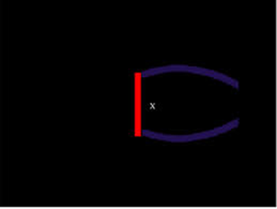
It is hard to see the blue arcs if you do not know what to look for, therefore I added a small visualization
A rough approximation of the Purkinje Blue Arcs
I can’t see it?!
Maybe you flipped your phone (or closed the wrong eye ;)) – be sure that the straight line points to the right
Maybe the room is still too bright. Also be sure that the red-color of the stimulus doesnt brighten up the background of the room
I don’t have an OLED screen: The demonstration should also work with just a red dot – maybe you have one at your stereo? Any bright red LED should work, the effect is smaller but still there. Your mileage on an LCD screen will vary…
What’s going on?
The nerve fibers from the photoreceptors are bundled and leave the retina through the optic discs. These nervebundles are called the Raphe. As visible in the next screen, Purkinjes Blue Arc follow the raphe perfect.y
The Raphe – all pointing towards the optical disc (Blind Spot)
Why exactly such a red bright stimulus activates the blue ganglio cells is currently not know.
I just started dabbling with Pluto.jl and very quickly it allows to give very insightful notebooks.
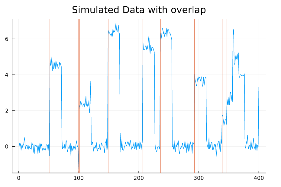
For example, take this signal:
X in samples, y in “µV”, blue = 1 EEG channel, orange= event onsets
Clearly, the simulated event-responses (the event-related potentials) overlap in time (e.g. at ~sample 350). We could do a “naive” regression on all timepoints relative to the event-onset, ignoring any overlap – or we could use linear deconvolution aka. overlap-correction to correct for the overlap (as the name says ;).
What follows is the beauty of Pluto.jl – simple reactive/interactive notebooks. As shown in the following gif, it is very easy to show the dependency of deconvolution-success on window-size and noise:
Mass Univariate analysis on the left, deconvolution on the right
Looks pretty robust for this simulation! Cool!
If you want to try for yourself: here is the notebook and here the link to the Unfold.jl toolbox
For my new EEG course in Stuttgart I spend some time to make this gif – I couldn’t find a version online. It shows a simple fact: If you calculate the mean, the breakdown point of 0%. That is, every datapoint counts whether it is an outlier or not. Trimmed or winsorized means instead calculate the mean based on the inner X % (e.g. inner 80% for trimmed mean of 20%, removing the top and bottom 10% of datapoints) – or in case of winsorizing the mean with the 20% extreme values not removed, but changed to the now new remaining limits). Therefore they have breaking points of X% too – making them robust to outliers.
Fun fact: a 100% trimmed mean is just the median!
As you can see, increasing the amount of outliers has a clear influence on the mean but not the 20% trimmed mean.
One important point: While sometimes outlier removal and robust statistics are very important, and arguable a better default (compared to mean) – you should also always try to understand where the outliers you remove actually come from.
The source code to generate the animation is here:
using Plots
using Random
using StatsBase

anim = @animate  for i ∈ [range(3,20,step=0.5)...,range(20,3,step=-0.5)...]
    Random.seed!(1);

    x = randn(50);
    append!(x,randn(5) .+ i); #add the offset

    histogram(x,bins=range(-3,20,step=0.25),ylims=(0,9.),legend=false)

    vline!([mean(x)],linewidth=4.)
    vline!([mean(trim(x,prop=0.2))],linewidth=4.)
    #vline!([mean(winsor(x,prop=0.2))])# same as trimmean in this example

end
gif(anim, "outlier_animation.gif", fps = 4)
I will be starting a new lab on Computational Cognitive Science, next month at University of Stuttgart. I will be working on the connection of EEG and Eye-Tracking, Statistics and methods development. The group is attached to the SimTech and the VIS Stuttgart
I recently asked on twitter whether people can recommend recording chambers to seat the subject in psychological experiments. I had a tough time googling it, terms that could be helpful in case you are in search for the same thing: Testing chamber, subject booth, audiology.
I got a lot of answers and for the sake of “google-ability” will summarize them here:
Steve Luck recommends a separated chamber, but highlights importance of air-conditioning due to sweating artefacts
Aina Puce recommends no chamber, but to sit 2-3m behind the subject and use white noise generators
Regarding actual chambers several commercial vendors were thrown in the ring:
Studiobricks*
Whisper Rooms*
Desone
Eckel
IAC Acoustics
* no Farraday cage directly available as far as I know. But check this tweet for a custom solution
I haven’t asked all vendors for a price estimate, but as far as I can tell, with climate control & lighting a ~4m² room costs around 8.000€ – 12.000€ without a Farraday Cage. With a cage I would guesstimate +10.00-15.000€ but I actually don’t really know.
PS: For this project I moved from EEG to fMRI, and in this post I will sometimes explain terms that might be very basic to fMRI people, but maybe not for EEG people.
I want to investigate cortical area V1. But I don’t want to spend time on retinotopy during my recording session. Thus I looked a bit into automatic methods to estimate it from segmented (segment = split up in WhiteMatter/GrayMatter+extract 3D-surfaces from voxel-MRI and also inflate them) brains. I used the freesurfer/label/lh.V1 labels and the neurophythy/Benson et al tools . The manual retinotopy was performed by Sam Lawrence using MrVista. And here the trouble begins:
The manual retinotopy was available only as a volume (voxel-file, maybe due to my completly lacking mrVista skills. I should look into whether I can extract the mrVista mesh-files somehow), while the other outputs I have as freesurfer vertex values, ready to be plotted against the different surfaces freesurfer calculated (e.g. white matter, pial (gray matter), inflated). Thus I had to map the volume to surface. Sounds easy – something that is straight forward – or so I thought.
After a lot of trial&error and bugging colleagues at the Donders, I settled for the nipype call to mri_vol2surf from freesurfer. But it took me a long time to figure out what the options actually mean. This answer by Doug Greve was helpful (the answer is 12 years old, nobody added it to the help :() (see also this answer):
It should be in the help (reprinted below). Smaller delta is better
but takes longer. With big functional voxels, I would not agonize too
much over making delta real small as you'll just hit the same voxel
multiple times. .25 is probably sufficient.

doug

   --projfrac-avg min max delta
   --projdist-avg min max delta

     Same idea as --projfrac and --projdist, but sample at each of the
     points    between min and max at a spacing of delta. The samples are then
     averaged    together. The idea here is to average along the normal.
The problem is that you have to map each vertex to a voxel. So in this approach you take the normal vector of the surface (e.g. from white matter surface), check where it hits the gray matter, sample ‘delta’ steps between WM (min) and GM (max), and check which voxels are closest to these steps. The average value of the voxels is then assigned to this vertex.
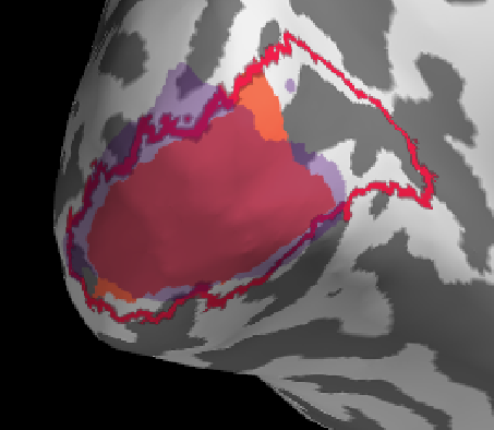
I will first show a ‘successful subject before I dive into some troubles along the way.
red=freesurfer label, orange = benson label restricted to <10deg visual angle, purple = manual based on 10deg retinotopy data
Overall a good match I would say, generally benson & freesurfer have a good alignment (reasonable), the manual retinotopy is larger in most subjects. This might also be due to the projection method (see below)
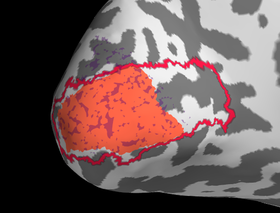
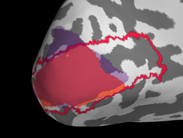
Initially I tried projection withour smoothing, see the results below. I then changed to a smooth of 5mm kernel with subsequent thresholding (for sure there is probably a smarter way).
It is pretty clear that in this example the fit of manual with automatic tools is not very good. My trouble is now that I don’t know if this is because of actual difference or because of the projection.
Next steps would be to double check everything in voxel land, i.e. project the surface-labels back to voxels and investigate the voxel-by-voxel ROIs.
22.10.2019 Edit: Thanks Matt Craddock, I understand the source of the problem better. He mentioned that this should not occur if the amplifiers record the triggers as trigger channels (before converting it to events). And mentions that this could happen through downsampling. Indeed after checking in the dataset I used it was downsampled from 1024 to 512Hz. This made many eventlatencies ~ X.50001, which will be uprounded with round and floored with floor. This gives some context to the problem. Full discussion on twitter
TLDR; EEGlab allows for non-integer event latencies (in units of samples). Eeglab chose floor(latency), while others e.g. unfold & fieldtrip choose round(latency) to round the latency to samples. This leads to differences between toolboxes, in my example of up to 1.5µV (or ~25% ERP magnitude). Importantly, this probably does not introduce bias between conditions
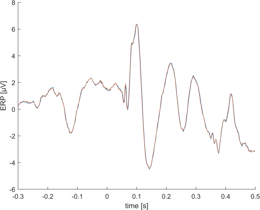
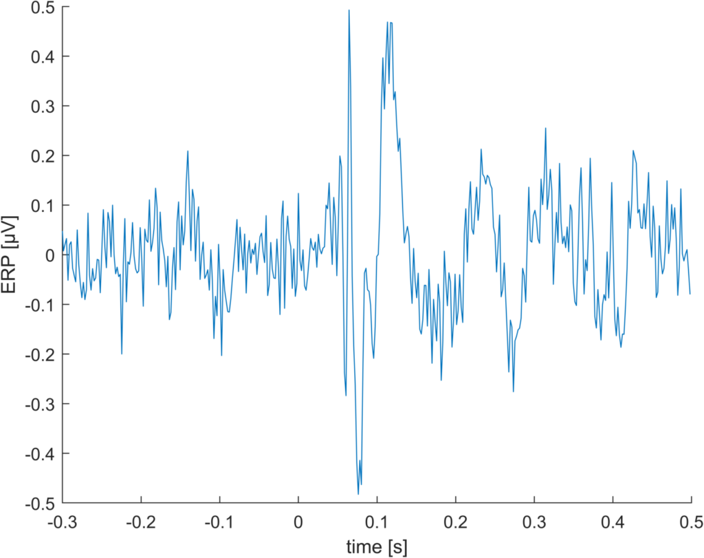
This is an ERP, actually its two ERPs. One is calculated using the “unfold” toolbox and one using eeglab’s pop_epoch function
Elec: PO8, average reference, 1280 trials, 512Hz, very typical experiment with single stimulus presentation, no task
If you look very closely, you can see that they are not identical, even though they should be. So – whats the difference?
It turns out that EEGlab saves event latencies in samples (e.g. stimulus is starting at sample 213), but also allows non-integer latencies (e.g. stimulus is starting between 212 and 213, to be exact: at sample 212.7). This makes sense, i.e. if your EEG sampling resolution is 100Hz you might know your stimulus onset with higher precision and not in 10ms bins. But in order to get ERPs we have to “cut” the signal at the event onset. EEGlab uses “floor” for this and rounds the stimulus onset from 212.7 to sample 212. Other toolboxes (unfold / fieldtrip) use “round”, thus the event would start at sample 213.
It turns out that in the example you see above, this introduces a difference between the two ERPs of 0.5µV (!) thats around 8% of the magnitude.
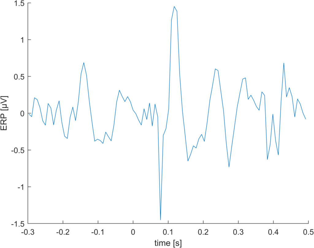
difference “floor” vs “round” for 512Hz data
This is just a random example I stumbled upon. With lower sampling rates, this effect should increase. Indeed, downsampling to 128 Hz gives us a whopping difference of 1.5µV.
Difference “floor”-“round” for 128Hz sampling rate
Floor vs. round (vs. others?)
The benefit of floor, at least the one I can think of, is that it would never shift the onset of a stimulus in the future. That is, it is causal. Possibly there are other benefits I am not aware of.
The benefit of round is that it more accurately reflects the actual stimulus onset. Possibly there are other benefits I am not aware of
Given that we mostly use acausal filtering anyway, I think the causal benefit is not very strong.
There is yet another alternative: a weighted average between samples. We could “split” the event onset to two samples, i.e. if we want the instantaneous stim-onset response, and stim onset is at sample 12.3, then sample 12 should be weighted 30% and sample 13 by 70%. I have to explore this idea a bit more, but I think its very easy to implement in unfold and test. But this for a new blogpost.
The big picture
In the fMRI community there are papers from time to time reporting that different analysis tools (or versions) lead to different results. I am not aware of any such paper in the EEG community (if you know one, let me know please!) but I think it would be nice if somebody would do such comparisons.
I currently do not forsee if such an event-latency-rounding difference could possibly introduce bias in condition differences. But I forsee that changing it will be difficult for the EEGlab developers, as “floor” has been around for a very long time in eeglab.
Code
Note that I did not use simulation here (but could have, it should be straight) but I cannot publicly share the data at this point in time.
I just gave my lecture at the Donders Toolkit. Many cool and interesting questions! I wish I had two hours, I had to skip some things I was excited about in favour of solid basics.
In case you are interested in other EEG slides, here are slides on overlap correction (deconvolution) and non-linear modeling (pptx, 8mb), an introduction to linear models (pptx, 50mb), and slides on multiple comparison corrections (pptx, 5mb)
Can’t give a proper license unfortunately, as some slides are based on old Donder Toolkit Slides, handed down from the years. All other authors I stole slides should be acknowledge, hope I did not forget something. Do as you wish with the slides. May the copywrite gods see favourable on our educator souls
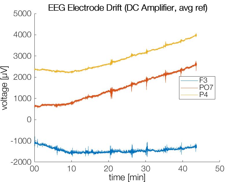
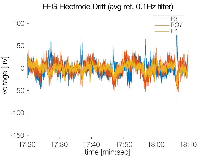
I coudn’t find an image of electrode drift for my slides, so here I quickly generated one. The only fancy thing is the usage of datetime to have minutes on the x-axis (I also made this post so I don’t forget this trick ;))
DC-Amplifier (REFA-2, tmsi) plot of three electrodes over ~45min recording data. Strong DC-Offsets and drifts are observed (this is typical & normal)
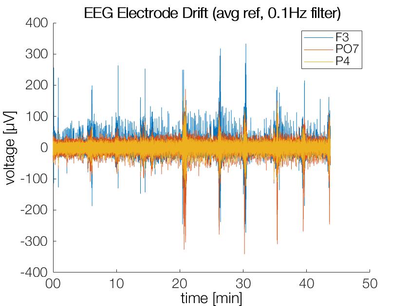
After filtering at 0.1Hz the strong drifts and offsets are gone (as intended), the y-axis has a very different axis now!
Obviously a cutoff-freq of 0.05Hz in the filter will still allow for some slow moving drifts. These offsets are usually accomodated for by baseline corrections
Thanks to Anna Lisa Gert for this dataset
% Load Data
EEG = pop_loadeep_v4('subj23.cnt');
% Load filtered data (takes 35min to filter...)
EEG_filt = pop_loadset('2_subj23_lowpass_resample_deblank.set');
%%
% Convert time to actual time
timesnew = datetime(EEG.times/1000,'ConvertFrom','epochtime','Epoch','2000-01-01');
% select random channels
chix = [5,63,27];

% Plot the unfiltered data
plot(timesnew,EEG.data(chix,:)')
% Make the plot beautiful
datetick('x','MM','keeplimits','keepticks') % only show minutes
xlabel('time [min]')
ylabel('voltage [µV]')
legend({EEG.chanlocs(chix).labels},'Location','East')
box off
title('EEG Electrode Drift (DC Amplifier, avg ref)')
set(gca,'fontsize', 14) % for a presentation
set(gca, 'FontName', 'HelveticaNeueLT Pro 45 Lt')
%%
% Convert again because data have been resampled
timesnew = datetime(EEG_filt.times/1000,'ConvertFrom','epochtime','Epoch','2000-01-01');

plot(timesnew,EEG_filt.data(chix,:)')

datetick('x','MM','keeplimits','keepticks')
xlabel('time [min]')
ylabel('voltage [µV]')
legend({EEG.chanlocs(chix).labels})
box off
title('EEG Electrode Drift (avg ref, 0.1Hz filter)')
set(gca,'fontsize', 14) % for a presentation
set(gca, 'FontName', 'HelveticaNeueLT Pro 45 Lt')
We move our eyes about four times per second, which is more often than our heart beats! Many studie show that these eye movements are a window into our minds (e.g. König et al. 2017) and are commonly used for basic research, marketing research and clinical assesments.
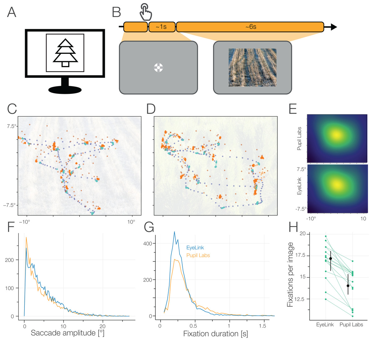
Even though eyetrackers are so commonly used and so powerful, they are rarely tested for how well they perform besides the manufacturers. Even more critical, no test battery existed before we set out on this project. Together with Katharina Groß (and Inga Ibs and Peter König) we developed a new eye tracker test battery which included most of the typically studied eye movements.
We chose to test two popular eye trackers concurrently: The Eyelink 1000 and the Pupil Labs glasses. The former is the working horse of eye movement research (release 2005), the latter the open hardware/source innovator (release 2014).
Our study reveals some strengths and some weakenesses for both eye trackers, but also of our newly proposed test battery. The results are numerours, so I will only depict two tasks:
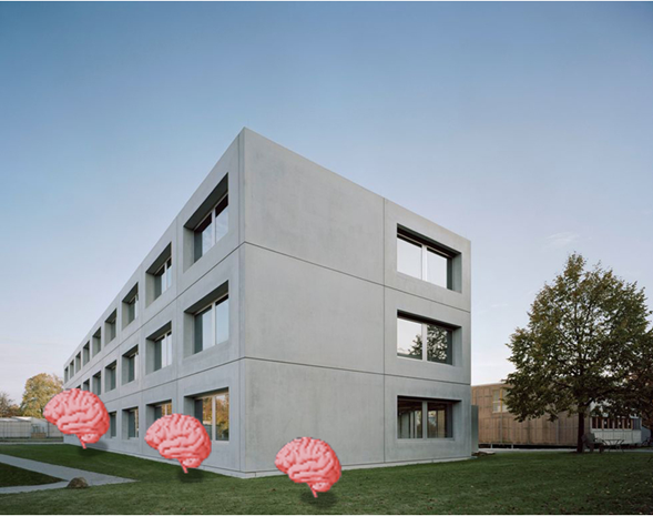
Free Viewing
Here you can see where a participant is looking on an image (C & D) with the task to simply explore the image. You can clearly see that the eye trackers agree on the coarse scale (blue & red dots kind of overlay), but not in the specific details (e.g. disagreements that worse/better at some locations. Also the red (pupil labs) eye-tracker has much higher variability during eye movements .
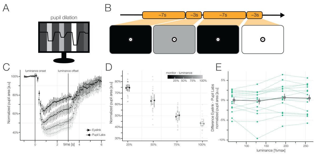
Pupil Dilation
Our pupil shrinks when it gets bright and opens up when it gets dark. We tested how well the eye tracker can measure this by presenting differently bright images interleaved by black images (so the pupil can go back (or near) to baseline). We found that on the average, both eye tracker give the same results (both eyetrackers are depicted on top of each other, barely differentiable in figure C) – but calculating the difference between eye trackers for each subject they differ quite a bit (green lines in E are not at 0%)!
Take home
Eye tracking scientists need information about the reliability and performance of their equipment to make informed decisions
Every eye movement has their own parameters to check for, e.g. pupil dilation has different requirements to an eye tracker than microsaccade research
That concludes this short laypersons summary. If you have any question feel free to comment here, write me, Katharina Groß, or any of my other co-authors. (paper doi: https://doi.org/10.7717/peerj.7086 )