Posts by: behinger

Sun Grid Engine Command-Dump

Here in the institute we have a Sun Grid Engine available. It is a tool to post computing-jobs on other workspaces (we have I think up to 60 available). There are certain commands and things that I do regularly which I tend to forget after half a year, or which might be useful for orthes.

  • Show all jobs that are running on the grid
    qstat -u \* or alternativly for a single user qstat -u behinger
  • exclude a single computer/host from running a job
    qsub -l mem=5G,h=!computername.domain script.sh
    to exclude multiple hosts: h=!h4&!h5 or h=!(h4|h5) Source
    of course mem=5G is an arbitrary other requirement.
  • Run a gridjob on a single R-File
    add #!/usr/bin/Rscript in the beginning of the file, then you can simply run qsub Rscript_name.R. I had problems using qsub Rscript -e "Rscript_name.R" due to the many quotes that would need escaping (I use to call the grid using system() command in matlab/R).

Matlab winsorized mean over all dimension

This is a function I wrote back in 2014. I think it illustrates an advanced functionality in matlab that I hadn’t found written about before.

The problem:

Calculate the winsorized mean of a multidimensional matrix over an arbitrary dimension.

Winsorized Mean

The benefits of the winsorized mean can be seen here:
Unbenannt-3

We replace the top 10% and bottom 10% by the remaining most extreme value before calculating the mean (left panel). The right panel shows how the mean is influenced by a single outlier, but the winsorized mean is not (ignore the “yuen”-box”)

Current Implementation

I adapted an implementation from the LIMO toolbox based on Original Code from Prof. patrick J Bennett, McMaster University. In this code the dimension is fixed at dim = 3, the third dimension.

They solve it in three steps:

  1. sort the matrix along dimension 3
  2. [matlab] xsort=sort(x,3); [/matlab]
  3. replace the upper and lower 10% by the remaining extreme value
  4. [matlab] % number of items to winsorize and trim
    g=floor((percent/100)*n);
    wx(:,:,1:g+1)=repmat(xsort(:,:,g+1),[1 1 g+1]);
    wx(:,:,n-g:end)=repmat(xsort(:,:,n-g),[1 1 g+1]);
    [/matlab]
  5. calculate the mean over the sorted matrix
  6. [matlab]wvarx=var(wx,0,3);[/matlab]

Generalisation

To generalize this to any dimension I have seen two previous solution that feels unsatisfied:
– Implement it for up to X dimension hardcoded and then use a switch-case to get the solution for the case.
– use permute to reorder the array and then go for the first dimension (which can be slow depending on the array)

Let’s solve it for X = 20 x 10 x 5 x 2 over the third dimension
[matlab]

function [x] = winMean(x,dim,percent)
% x = matrix of arbitrary dimension
% dim = dimension to calculate the winsorized mean over
% percent = default 20, how strong to winsorize

% How long is the matrix in our required dimension
n=size(x,dim);
% number of items to winsorize and trim
g=floor((percent/100)*n);
x=sort(x,dim);

[/matlab] up to here it my and the original version are very similar. The hardest part is to generalize the part, where the entries are overwritten without doing it in a loop.
We are now using the subsasgn command and subsref
We need to generate a structure that mimics the syntax of
[matlab] x(:,:,1:g+1,:) = y [/matlab] for arbitrary dimensions and we need to construct y

[matlab] % Prepare Structs
Srep.type = ‘()’;
S.type = ‘()’;

% replace the left hand side
nDim = length(size(x));

beforeColons = num2cell(repmat(‘:’,dim-1,1));
afterColons = num2cell(repmat(‘:’,nDim-dim,1));
Srep.subs = {beforeColons{:} [g+1] afterColons{:}};
S.subs = {beforeColons{:} [1:g+1] afterColons{:}};
x = subsasgn(x,S,repmat(subsref(x,Srep),[ones(1,dim-1) g+1 ones(1,nDim-dim)])); % general case
[/matlab] The output of Srep is:

Srep =
type: ‘()’
subs: {‘:’ ‘:’ [2] ‘:’ }

thus subsref(x,Srep) outputs what x(:,:,2,:) would output. And then we need to repmat it, to fit the number of elements we replace by the winsorizing method.

This is put into subsasgn, where the S here is :

Srep =
type: ‘()’
subs: {‘:’ ‘:’ [1 2] ‘:’ }

Thus equivalent to x(:,:,[1 2],:).
The evaluated structure then is:
[matlab] x(:,:,[1:2]) = repmat(x[:,:,1],[1 1 2 1]) [/matlab]

The upper percentile is replaced analogous:
[matlab] % replace the right hand side
Srep.subs = {beforeColons{:} [n-g] afterColons{:}};
S.subs = {beforeColons{:} [n-g:size(x,dim)] afterColons{:}};

x = subsasgn(x,S,repmat(subsref(x,Srep),[ones(1,dim-1) g+1 ones(1,nDim-dim)])); % general case

[/matlab]

And in the end we can take the mean, var, nanmean or whatever we need:
[matlab] x = squeeze(nanmean(x,dim));
[/matlab]

That finishes the implementation.

Timing

But how about speed? I thus generated a random matrix of 200 x 10000 x 5 and measured the timing (n=100 runs) of the original limo implementation and mine:

algorithm timing (95% bootstraped CI of mean)
limo_winmean 185 – 188 ms
my_winmean 202 – 203ms
limo_winmean otherDimension than 3    218 – 228 ms

For the last comparison I permuted the array prior to calculating the winsorized mean, thus the overhead. In my experience, the overhead is greater the larger the arrays are (I’m talking about 5-10GB matrices here).

Conclusion

My generalization seems to work fine. As expected it is slower than the hardcoded version. But it is faster than permuting the whole array.

Bayesian Modelling of Melanopsin

Bayesian Modelling of Melanopsin

Proccess
60%
In this project we work with Melanopsin, a photoactive opsin that can be used for optogenetical experiments. This is collaborative work with the Herlitze Lab from the Ruhr-Universität Bochum. A first paper got recently accepted in Current Biology which characterizes two different melopsin subtypes. The first version of our modeling work has recently been published on bioRxiv (preprint). The manuscript is work in progress, I’m very interested in discussing our approach and the manuscript.

Benedikt V. Ehinger¹, Dennis Eickelbeck², Katharina Spoida², Stefan Herlitze², Peter König¹³

Affiliations

¹Institute of Cognitive Science, University of Osnabrück, Albrechtstr. 28, 49076 Osnabrück, Germany
²Department of General Zoology and Neurobiology, ND7/31, Ruhr-University Bochum, Universitätsstr. 150, D-44780 Bochum, Germany
³Dept. of Neurophysiology and Pathophysiology, University Medical Center Hamburg Eppendorf, 20246 Hamburg, Germany

Predictive Coding in the Blind Spot

Predictive Coding in the Blind Spot

Project Done
100%
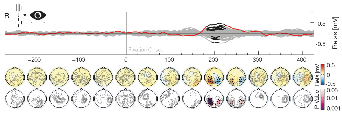
We investigate the blind spot in an online gaze-dependent eyetracking / EEG paradigm. We recently published our findings in the Journal of Neuroscience. We also gave a talk at the Vision Science Society. We had posters at the Statistical Challenges Conference in Warwick, the Donders-Discussions in Nijmegen and the Brain-Conference in Kopenhagen in May. We further had great Posters at the ECEM in Vienna and the MMN conference in Leipzig. I love to discuss our work on the blind spot and the resulting prediction errors and implications for predictive coding with you!

Benedikt V. Ehinger¹, Peter König¹², Josè Ossandon¹

Affiliations

¹ Institute of Cognitive Science, University of Osnabrück
² Institut für Neurophysiologie und Pathophysiologie, UKE Hamburg


Walk the Line

Walk the Line

Project Done
100%

This project was winner of the one week student project competition at the BCBT 2012 summer school.

Authors

Benedikt V. Ehinger, University of Osnabrück
Anna L. Gert, University of Osnabrück
Andrew Martin, Goldsmiths, University of London
Sasa Bodiroza, HU Berlin
Giovanni Maffei, Universitat Pompeu Fabra
Guido Schillac, HU Berlin
Alex Maye, UKE Hamburg

Planning: BE,AG,AnM,SB,GM,GS,AlM. Pilot Recording & Analysis: BE,AG. Programming: AnM,SB,GM. Recordings: AG,AnM,SB,GM,GS. Anaylsis BE, AG. Text/Presentation: BE, AG, AnM


Introduction:

Not many studies exist, that measure deviation of subjects while walking an ideal line while beeing blindfolded. This study tries to gather data and get an estimate, how big the deviation at the end of a 3m walk is. We also try to modulate our subjects performance with adding online auditory feedback. We hypothesize that performance with visual feedback is near perfect, blind performance has a significant deviation, while auditory feedback helps the subject

Visual Category Learning

Visual Category Learning

Project Done
100%

We observe learning of novel classes of perceptual stimuli in an M/EEG study over more than 20 sessions.

Authors

Benedikt V. Ehinger, Danja Porada, Andreas Engel, Peter König, Tim C. Kietzmann

Introduction

Everyday we use categories to interpret and act on our environment. Of course, this is necessary as we have to discriminate for example edible from poisonous food or friend from foe. Such representations are involuntarily and immediately accessible to our consciousness. How do new categories emerge in our brain? One way to study human category behaviour is to train humans to learn new classes by presenting different stimuli with some kind of feedback and analyse their behaviour. In addition to observing patterns of behaviour, electroencephalography (EEG) can be used to study the evoked electrical changes by different category based tasks in the brain.
Due to low level confounds, we see that a categorizing process into two categories is hard to distinguish from other neuronal processes. Therefore we need to find another paradigm to examine this process. We use an adaptation approach (c.f. Grill-Spector, Henson and Martin (2006)). This adaptation effect is used in various contexts, for example in fMRI, to distinguish different neuronal populations (Krekelberg, Boynton, van Wezel. 2006) or, as in our experiment, as a measurement of category membership.

7 of 7
1234567