Modelling Circular Effects using Splines

Note: This blog is just explaining the basis sets, not how to actually fit models / get parameters etc.

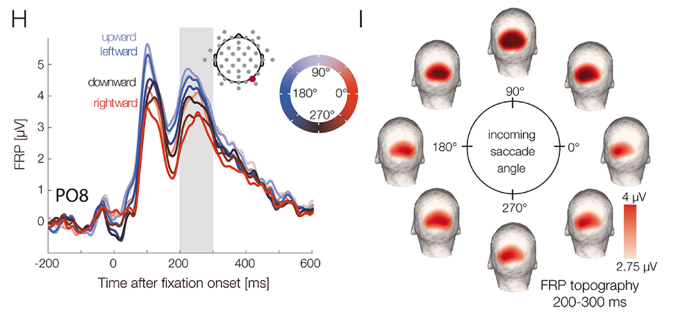
Recently, we used the unfoldtoolbox (Matlab or Julia; access it from python!) to analyze some fixation-related ERPs. The approach we used (multiple regression with deconvolution) allowed us to include this circular-predictor: absolute saccade-angle.

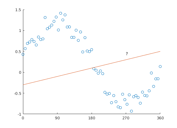
Why can’t we model saccade-angle using a linear predictor? The issue is straightforward: Look at this plot.

Ok, why can’t we use a standard non-linear spline regression?

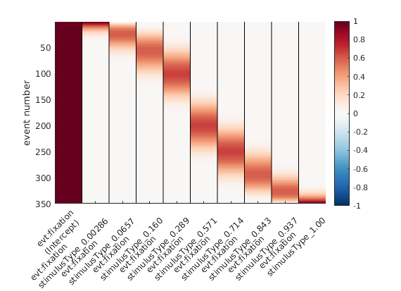
Wait – what even is a standard non-linear spline regression? Great that you asked. Instead of fitting a straight line with parameters slope & intercept (think y = m*x + c), we can split up the x-axis regressor in multiple “local” regressors.

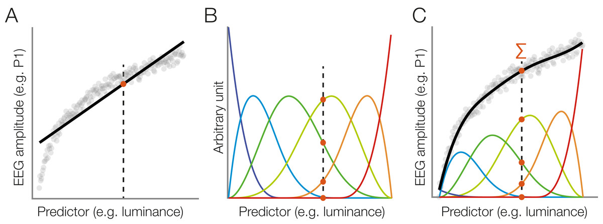
But: The angle starts at x=0, and goes to x=360 – but we all know, x=0 and x=360 are actually identical! The orange line added to the plot would have 0 & 360 at different values, except for a slope of 0.

How do we fix this, how do we “wrap around” the predictor axis?

Circular Splines!

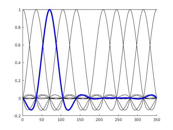
Instead of having basis functions that have bounds at 0 / 360°, we are using a basis function set that wraps the circular space. If the idea didn’t become clear, here is an alternative visualization:

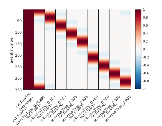
Hopefully, these visualizations help some of you to understand circular splines better!

Disclaimer: Thanks to Judith Schepers for discussing this with me; sorry for the typos etc. I am a bit in a rush