Simple Filter Generation

I sometimes explain concepts to my students. Then I forget the code and the next time round, I have to redo it. Take this post as an extended memory-post. In this case I showed what filter-ringing artefacts could look like. This is especially important for EEG preprocessing where filtering is a standard procedure.

A good introduction to filtering can be found in this slides by andreas widmann or this paper by andreas widmann

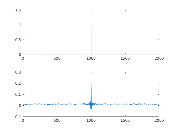
Impulse with noise

I simulated as simple impulse response with some additional noise. The idea is to show the student that big spikes in the EEG-data could result in filter-ringing that is quite substantial and far away from the spike.

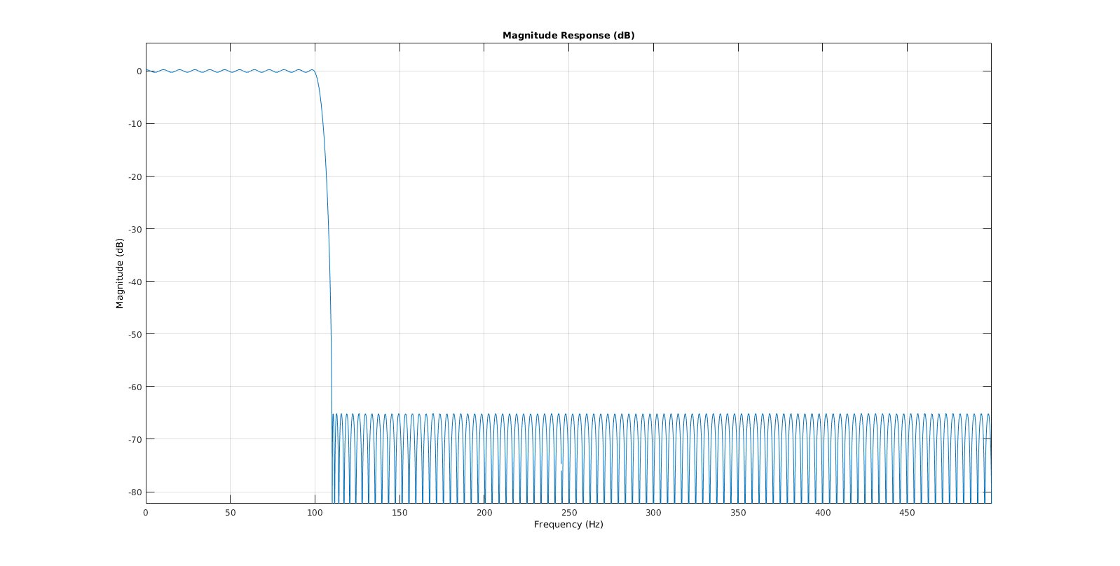
The filter

This is the filter I generated. It is a BAD filter. It shows huge passband ripples. But for educational purposes it suits me nice. I usually explain what passbands, transitionband, stopband, ripples and attenuation means.

The code

“`matlab
fs = 1000;
T = 2;
time = 0:1/fs:T-1/fs;

data = zeros(length(time),1);
% data(end/2:end) = data(end/2:end) + 1;
data(end/2) = data(end/2) + 1;
data = data + rand(size(data))*0.02;

subplot(2,1,1)
plot(data)

filtLow = designfilt(‘lowpassfir’,’PassbandFrequency’,100, …
‘StopbandFrequency’,110,’PassbandRipple’,0.5, …
‘StopbandAttenuation’,65,’SampleRate’,1000);

subplot(2,1,2)

% 0-padding to get the borders right
data = padarray(data,round(filtLow.filtord));

% Filter twice to get the same phase(non-causal)
a = filter(filtLow,data);
b = filter(filtLow,a(end:-1:1));
b = b(round(filtLow.filtord)+1:end – round(filtLow.filtord));
plot(b)

fvtool(filtLow) % to look at the filter

“`