LMM Type-1 Error for 1+condition+(1|subject)

Like Interactive Explorations?
Try out the interactive Type-1 errors LMMs Demo here

In repeated measures designs, we commonly repeat trials within a subject. This leaves us with a problem, though: trials from within one subject are typically more similar compared to trials across subjects. This requires us to use repeated-measures ANOVAs, Hierarchical, Multi-Level, or as in the case of this blog: Linear Mixed Models.

I commonly see analyses for within-subject designs with LMMs, that use formulas like:

y~1+condition+(1|subject)

or

y~1+condition+(1|subject) + (1|item)

Type-1 Error of omitting condition random slopes

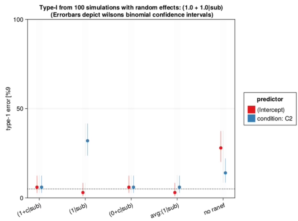
As can be seen in this graph, the type-1 error of omitting the random slope of subject can be huge, if such a slope is actually present in the data. The size of this type-1 error deviation depends on several things, most importantly the size of the random slope compared to the residual variability, but also the number of trials per subject, the number of subjects, residual variability and others.

The correct model to use is:

y~1+condition+(1+condition|subject)

(I think) the underlying thought is, that by using (1|subject), we allow each subject to have different values, thus the differences between subjects are accounted for. But this is too simplified. While we account for the general offset of each subject, we didn’t reach all the way – we forgot to take into account, that trials from a within-subject condition effects will be more similar to each other as well – not only the modelled Intercept-offset.

Indeed, this fallacy is addressed in many papers on LMMs, for instance in the famous “Keep it maximal” paper:

A common misconception is that crossing subjects and items in the intercept term of LMEMs is sufficient for meeting the assumption of conditional independence, and that including random slopes is strictly unnecessary […]. Indeed, some researchers have already warned against using random-intercepts-only models when random slope variation is present (e.g., Baayen, 2008; Jaeger, 2011a; Roland, 2009; Schielzeth & Forstmeier, 2009)

Barr et. al. 2013

A different motivation might be, that this is the only model that “converges”. Typically, some kind of model simplification is performed, removing correlations, then slopes, then intercepts (but why not remove intercepts before slopes?) Anyway, this leads us a bit astray to the domains of Matuschek 2019, who argue that always sticking to the maximal model has a cost in power (e.g. from 15% to 10% in small samples, or ~45% to 40% in middle sized samples; model-simplification vs. maximal model, Figure 1+2); while at the same time, they argue, the type-1 hit in that test region is small. Importantly, they never argue to start with the 1+(1|subject) model! While in some proportion of the simulations (up to 80% for very small datasets, Figure 3), this model is ultimately selected, they argue: “Our simulations showed that, in the long run, the parsimonious model yields the best chances to detect a true fixed effect as significant.” – but this includes their model-simplification procedure.

Intuition: Why is slope more important than intercept (to control type-1 of condition)?

One superficial way to think about this issue, is to think about the difference of (1|subj) and (1+c|subj): The former is a design where you record multiple trials from each subject, but for each subject only in one condition (condition between subject). In the latter, you record multiple trials from both conditions (within subject). It just seems intuitive to me, that these two very different designs, should be reflected by different models.

For the second way, we need an example: Let’s say, we recently invented the HairStretchShampoo^tm, but we don’t know if it actually works. Thus, we invite 100 subjects, each 20 times, and measure their hair length. Each time, they either applied the HairStretchShampoo^tm – or not. Our analysis model is:

hairlength~1+used_shampoo+(1+used_shampoo|subject)

or in pseudo-math notation where $\beta$ = fixed effects and $\theta$ = variances

hairlength = $\beta_{int} + \beta_{shamp} + (\theta_{int}+\theta_{shamp}|subject)$

The following components account for the following things (assuming effect coding):

• $\beta_{int}$ fixed intercept effect: 40cm. Accounts for the average hair length over all subjects.
• $\beta_{shamp}$ fixed shampoo effect: 1cm. Accounts for the average Shampoo-effect (this is what you want to know + it’s uncertainty).
• $\theta_{int}$ random intercept effect: SD = 20. Accounts for variation between subjects on their hair length, this will likely be rather large. It tells you, that the average hair length varies considerably around the fixed effect of 40cm.
• $\theta_{slope}$ random shampoo effect: SD = 2. How different does the shampoo work for different subjects? With an average fixed effect of 1cm, this SD tells you the shampoo works for some, but probably not all subjects.

_{Note: In the list above we are not interpreting uncertainties, that is Standard Errors, t- or p-values, but rather the actual estimated model components.}

If one would drop the $\theta_{slope}$ and model only the random intercept, what effectively happens is that one assumes the HairStretchShampoo^tm-effect is identical for all subjects – even though in our example above, we “know” it varies considerable (SD=2, around a small effect of 1cm). Further, such a model assumes that the repeated measures of condition (remember, 20 repeated measurements per subject) are actually coming from independent subjects and thus contain independent information

larger number of trials => larger degrees of freedom => smaller standard errors

Sidetrack: Don’t random intercepts explain more variance?
What you typically would notice, and is true in our example above, is that the Intercept fixed+random part explains much more variability in our data than the condition effect. The condition effects live “on-top” of that variability. Explaining variability in our data is generally a good thing. If we explain more variability, our uncertainty is reduced (smaller residuals => smaller SEs => smaller p-values). Thus, we should definitely care about including intercepts. But they do not make our repeated condition measurements independent.

Special cases and observations

1. If you only have one trial per condition-level, there is no way to differentiate the random slope variability from the residual variability. In that case, leaving the random slope does not lead to higher type-1 errors. In other words, if you average within subject your conditions first, then the random-intercept-only model (1|sub) is fine.
2. The (0+c|sub) performs pretty well. Indeed, Barr et al. also benchmark it and come to the same conclusion. I haven’t seen it in another paper, but they recommend dropping the intercept before the slope. That was new to me. Thus, the “ideal” way for model simplification as I see it now, is to: first drop correlation, then intercepts, then slopes of interests (except if any of those parameters is of interest). A PCA on the Random Effects (rePCA in Julia), might help identify what exactly is best to drop.
3. It was very surprising to me how little the presence of random-intercept mattered, if one is only interested in condition effect. This plays together with 2)
4. The whole thing generalizes to (1|sub)+(1|item) designs, as in Barr et al 2013 (seriously, go read that paper!)

I want to conclude with another quote from Barr et al:

This goes to show that, for such designs, crossing of random by-subject and by-item intercepts alone is clearly not enough to ensure proper generalization of experimental treatment effects (a misconception that is unfortunately rather common at present)

Barr et. al. 2013