Multitaper Time vs Frequency Resolution
Goal
Give a graphical representation of multitaper time frequency parameters.
Background
Frequency Resolution and sFFT
In M/EEG analysis we are often interested in oscillations. One tool to analyse oscillations is by using time-frequency methods. In principle they work by segmenting the signal of interest in small windows and calculating a spectrum for each window. A tutorial can be found on the fieldtrip page. There exists a time-frequency tradeof: $\delta f = \frac{1}{T}$ with T the timewindow (in s) and $\delta f$ the frequency resolution. The percentage-difference of two neighbouring frequency resolution gets smaller the higher the frequency goes, e.g. a $\delta f$ of 1 at 2Hz and 3Hz is 50%, but the same difference at 100Hz and 101Hz is only 1%. Thus usually we try to decrease the frequency resolution the higher we go. A popular examples are wavelets, they inherently do this. One problem with wavelets is, that the parameters are not perfectly intuitive (I find). I prefer to use short-time FFT, and a special flavour the Multitaper.
Multitaper
We can sacrifice time or frequency resolution for SNR. I.e. one can average estimates at neighbouring timewindows or estimates at neighbouring frequencies. A smart way to do this is to use multitapers, I will not go into details here. In the end, they allow us to average smartly over time or frequency.
Parameter one usually specifies
- foi: The frequencies of interest. Note that you can use arbitrary high resolution but if you have $\delta foi < \delta f$ then information will be displayed redundantly (but it looks smoother).
- tapsmofrq: How much frequency smoothing should happen at each foi.
- t_ftimwin: The timewindow for each foi
Plotting the parameters
With the matlab-function attached to the end of the post one can see the effective frequency-resolution of the parameters in a single plot. For this example I use the frequency parameters by Hipp 2011. They logarithmically scale up the frequencybandwith. In order to do so for the low frequencies (1-16Hz) they change the size of the timewindow, for the higher frequencies they use multitaper with a constant window size of 250ms.
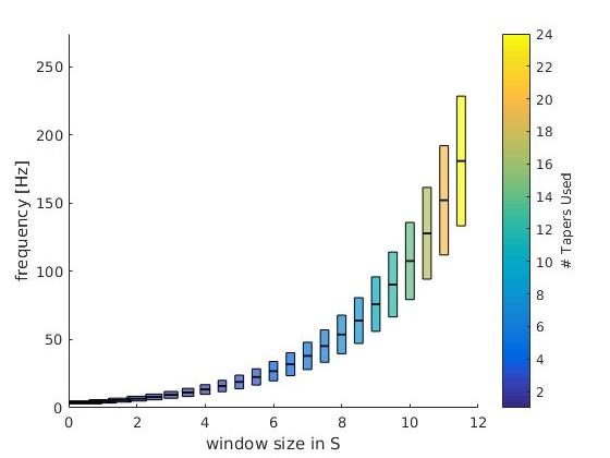
This is the theoretical resolution (interactive graph), i.e. a plot of the parameters you put in. foi +- tapsmofrq scaled by each timewindow size. Note: The individual bar size depicts the window-size of the respective frequency-bin.
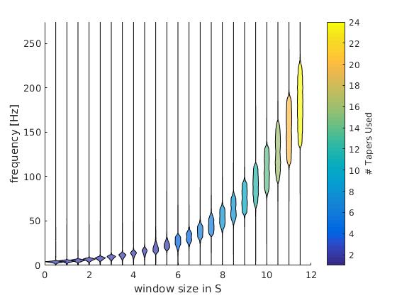
This is the numeric resolution (interactice graph). I used the frequency response of 100 repetitions of white noise (flat spectrum over repetitions) and calculated the frequency response of the multitaper filters. This is scaled in the x-axis by the time-window used.
Check out the interactive graphs to see how the time-windows change as intendet with lower frequencies.
The colorbar depict the number of tapers used. As intended, the number of tapers do not change from 1-16Hz.
Code
function [] = plot_taper(inpStruct,cfg)
%% plot_taper
% inpStruct: All fields need to have the same length
%   foi       : The frequencies of interest.
%   tapsmofrq : How much frequency smoothing should happen at each foi (+-tapsmofrq)
%   t_ftimwin : The timewindow for each foi
% You can also directly input a fieldtrip time-freq object
%
% cfg:
%   logy      : plot the y-axis as log10
%   type      : "theoretical" : This plots the foi+-tapsmofrq
%               "numerical"   : Simulation of white noise to approx the
%               effective resolution

if nargin == 1
    cfg = struct();
end

if isfield(cfg,'logy')
    assert(ismember(cfg.type,[0,1]),'logy has to be 0 or 1')
    logy = cfg.logy;
else
    logy = 0;
end
if isfield(cfg,'type')
    assert(ismember(cfg.type,{'numerical','theoretical'}),'type has to be ''numerical'' or ''theoretical''')
    type = cfg.type;

else
   type = 'numerical';
end
nRep = 100; % repetitions of the numeric condition
xscaling = 0.5;
if ~isempty(inpStruct) && isfield(inpStruct,'t_ftimwin')
    fprintf('cfg detected\n')
    cfg = inpStruct;
elseif ~isempty(inpStruct) && isfield(inpStruct,'cfg')
    fprintf('fieldtrip structure detected\n')
    cfg = inpStruct.cfg;
else
    fprintf('using parameters from Hipp 2010 Neuron \n')
    cfg =[];

    % we use logspaced frequencies from 4 to 181 Hz
    cfg.foi = logspace(log10(4),log10(181),23);

    % The windows should have 3/4 octave smoothing in frequency domain
    cfg.tapsmofrq = (cfg.foi*2^(3/4/2) - cfg.foi*2^(-3/4/2)) /2; % /2 because fieldtrip takes +- tapsmofrq

    % The timewindow should be so, that for freqs below 16, it results in n=1
    % Taper used, but for frequencies higher, it should be a constant 250ms.
    % To get the number of tapers we use:  round(cfg.tapsmofrq*2.*cfg.t_ftimwin-1)
    cfg.t_ftimwin = [2./(cfg.tapsmofrq(cfg.foi<16)*2),repmat(0.25,1,length(cfg.foi(cfg.foi>=16)))];
end

max_tapers = ceil(max(cfg.t_ftimwin.*cfg.tapsmofrq*2));
color_tapers = parula(max_tapers);
%%
figure
for fIdx = 1:length(cfg.t_ftimwin)
    timwin = cfg.t_ftimwin(fIdx);
    tapsmofrq = cfg.tapsmofrq(fIdx); % this is the fieldtrip standard, +- the taper frequency
    freqoi = cfg.foi(fIdx);
    switch type
        case 'theoretical'
            % This part simply plots the parameters as requested by the
            % user.
            y = ([freqoi-tapsmofrq freqoi+tapsmofrq freqoi+tapsmofrq freqoi-tapsmofrq]);

            ds = 0.3;
            ys = ([freqoi-ds freqoi+ds freqoi+ds freqoi-ds]);
            if logy
                y = log10(y);
                ys = log10(ys);
            end
            x = [-timwin/2 -timwin/2 +timwin/2 +timwin/2]+fIdx*xscaling;

            patch(x,y,color_tapers(round(2*timwin*tapsmofrq),:),'FaceAlpha',.7)
            patch(x,ys,[0.3 1 0.3],'FaceAlpha',.5)
        case 'numerical'
            fsample = 1000; % sample Fs
            % This part is copied together from ft_specest_mtmconvol
            timwinsample = round(timwin .* fsample); % the number of samples in the timewin

            % get the tapers
            tap = dpss(timwinsample, timwinsample .* (tapsmofrq ./ fsample))';
            tap = tap(1:(end-1), :); % the kill the last one because 'it is weird'

            % don't fully understand, something about keeping the phase
            anglein  = (-(timwinsample-1)/2 : (timwinsample-1)/2)'   .*  ((2.*pi./fsample) .* freqoi);

            % The general idea (I think) is that instead of windowing the
            % time-signal and shifting the wavelet per timestep, we can multiply the frequency representation of
            % wavelet and the frequency representation of the data. this
            % masks all non-interesting frequencies and we can go back to
            % timespace and select the portions of interest. In formula:
            % ifft(fft(signal).*fft(wavelet))
            %
            % here we generate the wavelets by windowing sin/cos with the
            % tapers. We then calculate the spectrum
            wltspctrm = [];
            for itap = 1:size(tap,1)
                coswav  = tap(itap,:) .* cos(anglein)';
                sinwav  = tap(itap,:) .* sin(anglein)';
                wavelet = complex(coswav, sinwav);
                % store the fft of the complex wavelet
                wltspctrm(itap,:) = fft(wavelet,[],2);
            end


%           % We do this nRep times because a single random vector does not
%           have a flat spectrum.
            datAll = nan(nRep,timwinsample);
            for rep = 1:nRep
                sig = randi([0 1],timwinsample,1)*2-1; %http://dsp.stackexchange.com/questions/13194/matlab-white-noise-with-flat-constant-power-spectrum
                spec = bsxfun(@times,fft(sig),wltspctrm'); % multiply the spectra
                datAll(rep,:) = sum(abs(spec),2); %save only the power
            end
            dat = mean(datAll); %average over reps


            % normalize the power
            dat = dat- min(dat);
            dat = dat./max(dat);

            t0 = 0 + fIdx*xscaling;
            t = t0 + dat*timwin/2;
            tNeg = t0 - dat*timwin/2;

            f = linspace(0,fsample-1/timwin,timwinsample);%0:1/timwin:fsample-1;
            if logy
                f = log10(f);
            end
            % this is a bit hacky violin plot, but looks good.
            patch([t tNeg(end:-1:1)],[f f(end:-1:1)],color_tapers(2*round(timwin*tapsmofrq),:),'FaceAlpha',.7)
    end


end
c= colorbar;colormap('parula')
c.Label.String = '# Tapers Used';
caxis([1 size(color_tapers,1)])

set(gca,'XTicks',[0,1])
xlabel('width of plot depicts window size in [s]')
if logy
    set(gca,'ylim',[0 log(max(1.2*(cfg.foi+cfg.tapsmofrq)))]);
    ylabel('frequency [log(Hz)]')
else
    set(gca,'ylim',[0 max(1.2*(cfg.foi+cfg.tapsmofrq))]);
    ylabel('frequency [Hz]')
end
end