Applied Generalized Linear (Mixed) Modelling
Benedikt Ehinger
March 19th, 2018
Athena: https://athena.cogsci.uos.de/
Please fill in the feedback after the second session

Course Overview
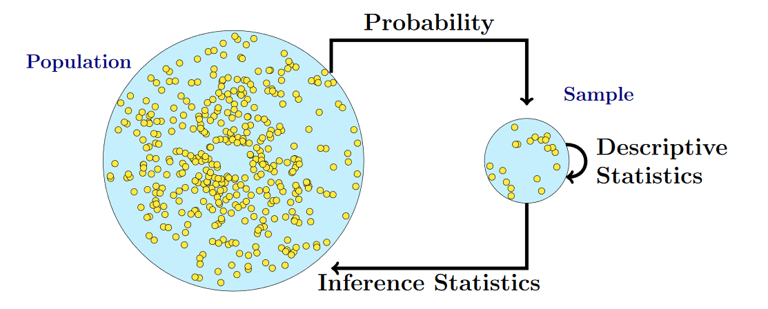
Purpose of statistics
- Organization

- Description
- Inference
Why statistics in the first place?
Because of Variation

Most important lesson
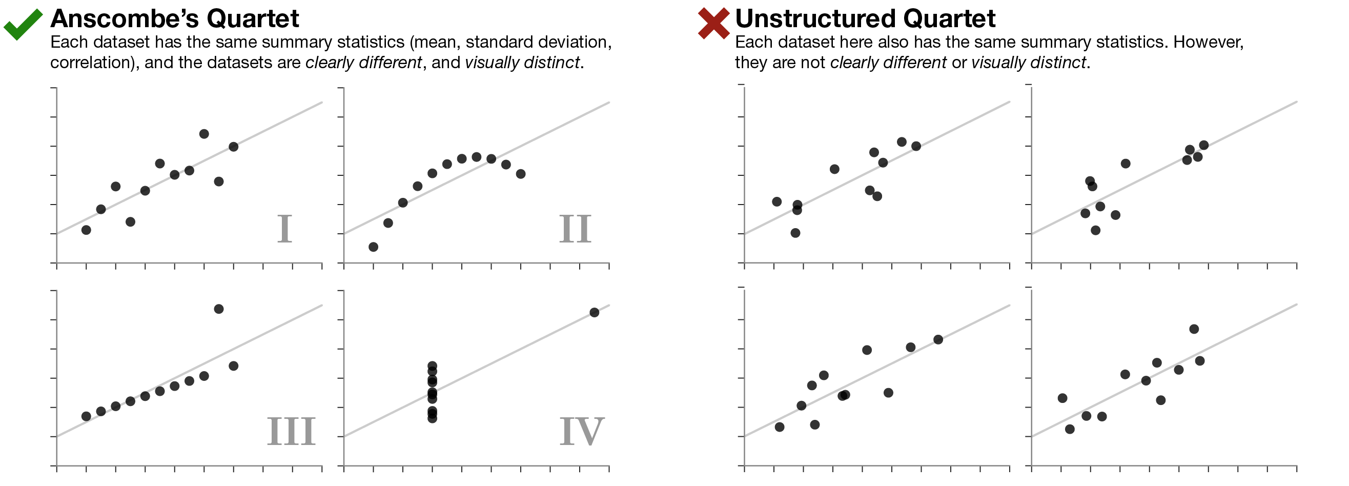
Always visualize your data
…make both calculations and graphs. Both sorts of output should be studied; each will contribute to understanding. F. J. Anscombe, 1973

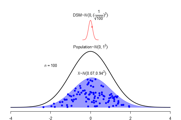
Population
This could be the height of the population
of all people in this room.
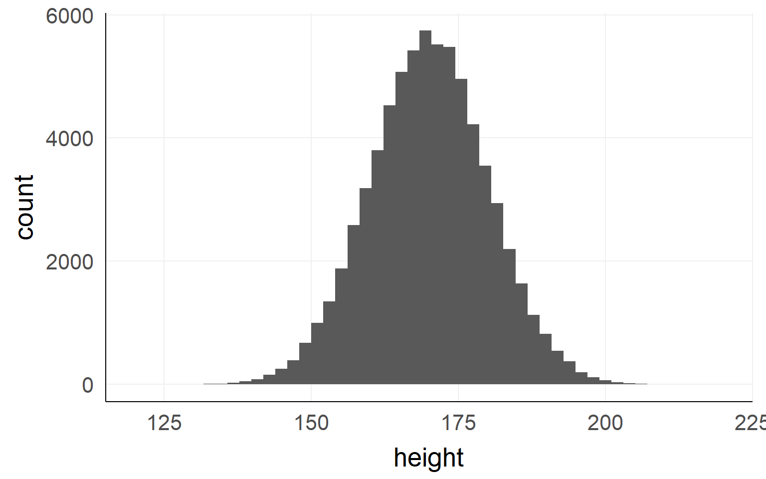
This could be the height of the population of all people in the world. The upper example is a sub-population.
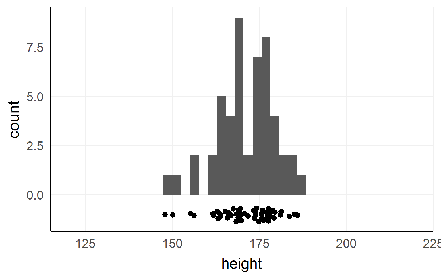
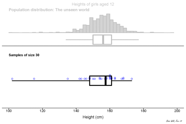
Sample
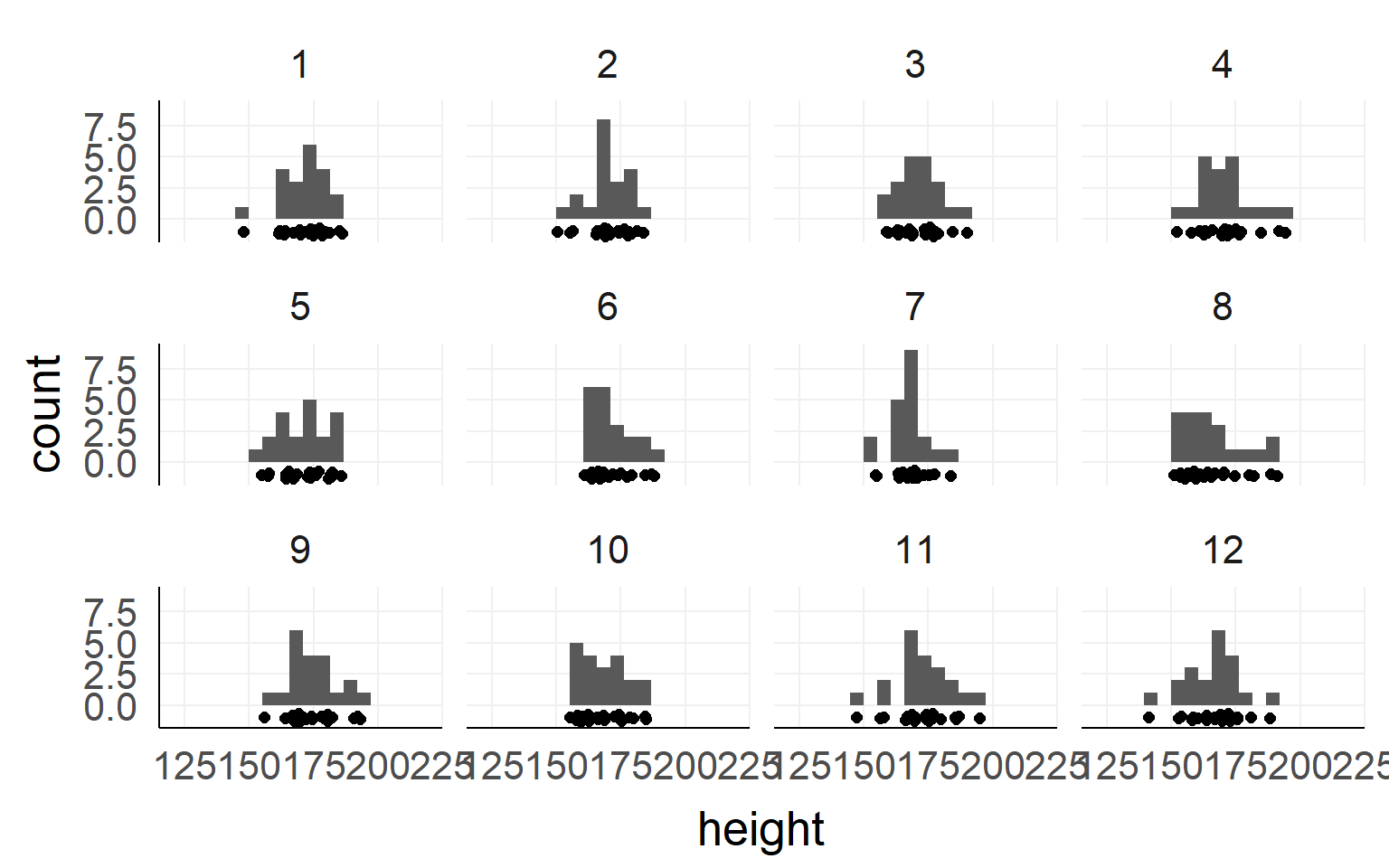
Height measured of 12 different samples (=experiment) of a population.
Sampling Distribution
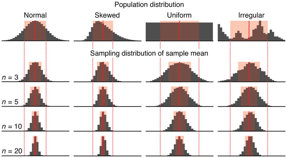
Central limit theorem
What are statistical inferences?
Example \(n_{obs} = 10\)
##  [1] -0.37645381  0.43364332 -0.58562861  1.84528080  0.57950777
##  [6] -0.57046838  0.73742905  0.98832471  0.82578135 -0.05538839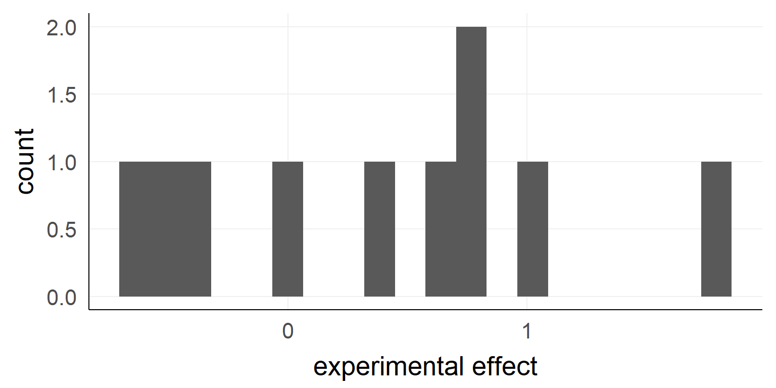
## [1] "mean:0.38, sd:0.78"The \(H_0\) model
Take 1000 random samples with \(n = n_{obs} = 10\) each
dnull =replicate(1000, rnorm(10) ) %>%reshape2::melt()
null_stat = dnull%>%group_by(Var2)%>%summarise(m = mean(value)) # var2 codes the sample-ID
qplot(null_stat$m,bins=50)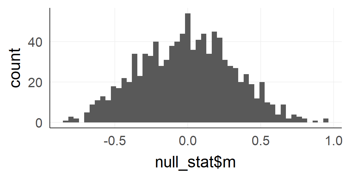
Q: What is this distribution called?
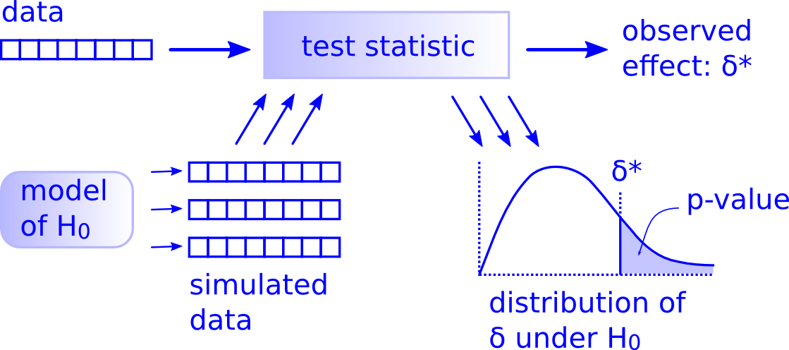
The p-value
Because standardization makes things comparable!
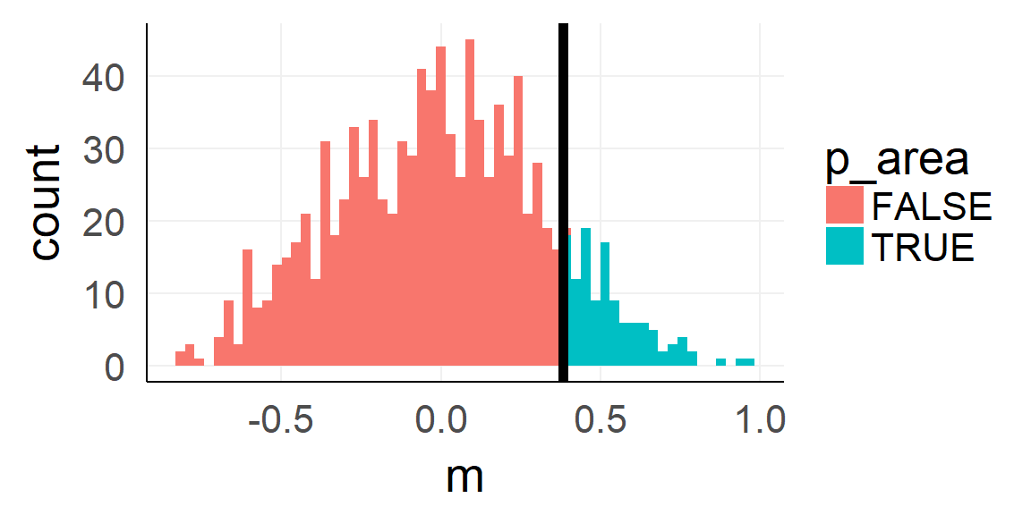
sprintf('p-value: %.3f',sum(null_stat$m >=mean(dobs)) / 1000)## [1] "p-value: 0.121"Analytic shortcut
Simulation can be expensive (e.g. in very complex models => day 4) and computers are needed.

For normal distributed populations (assumption!) the sampling distribution can be easily calculated (a normal with mean = \(mean_{H_0}\), \(SE = \frac{\sigma_{H_0}}{\sqrt N}\), Standard-error)
Summary
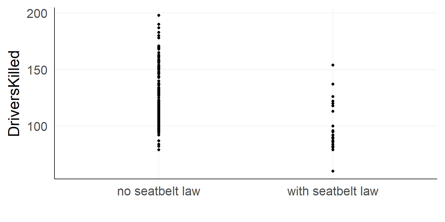
Should the seatbelt law be withdrawn?

ggplot(data,aes(x=law,y=DriversKilled))+stat_summary()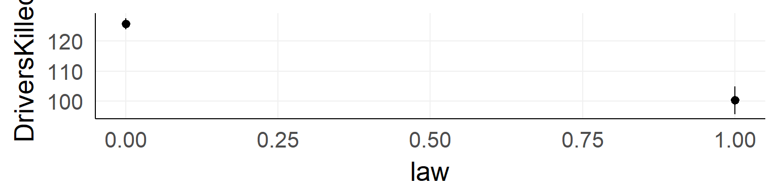
There could be confounds!
ggplot(data,aes(x=date,y=PetrolPrice,color=factor(law)))+geom_point()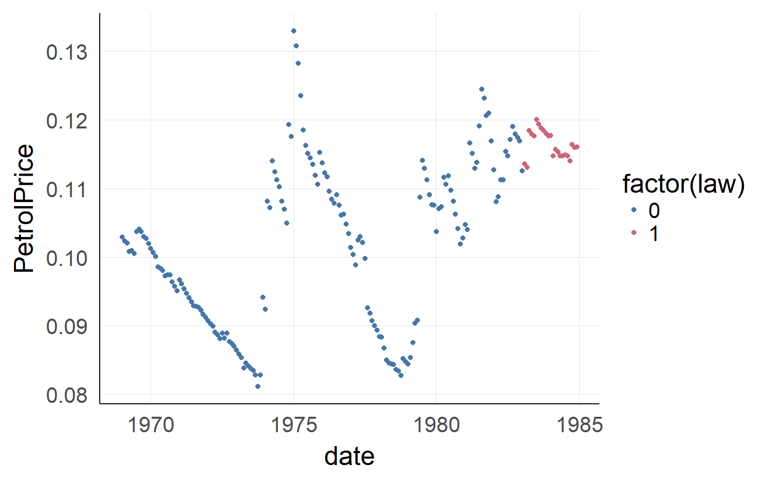 We will ignore the dependency in time. Please never do this in your data - this is an example only! You have been warned
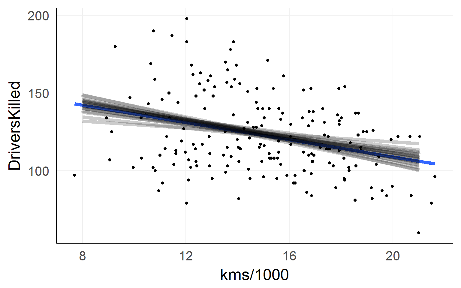
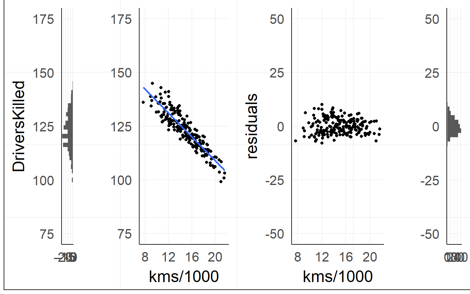
The simple linear regression
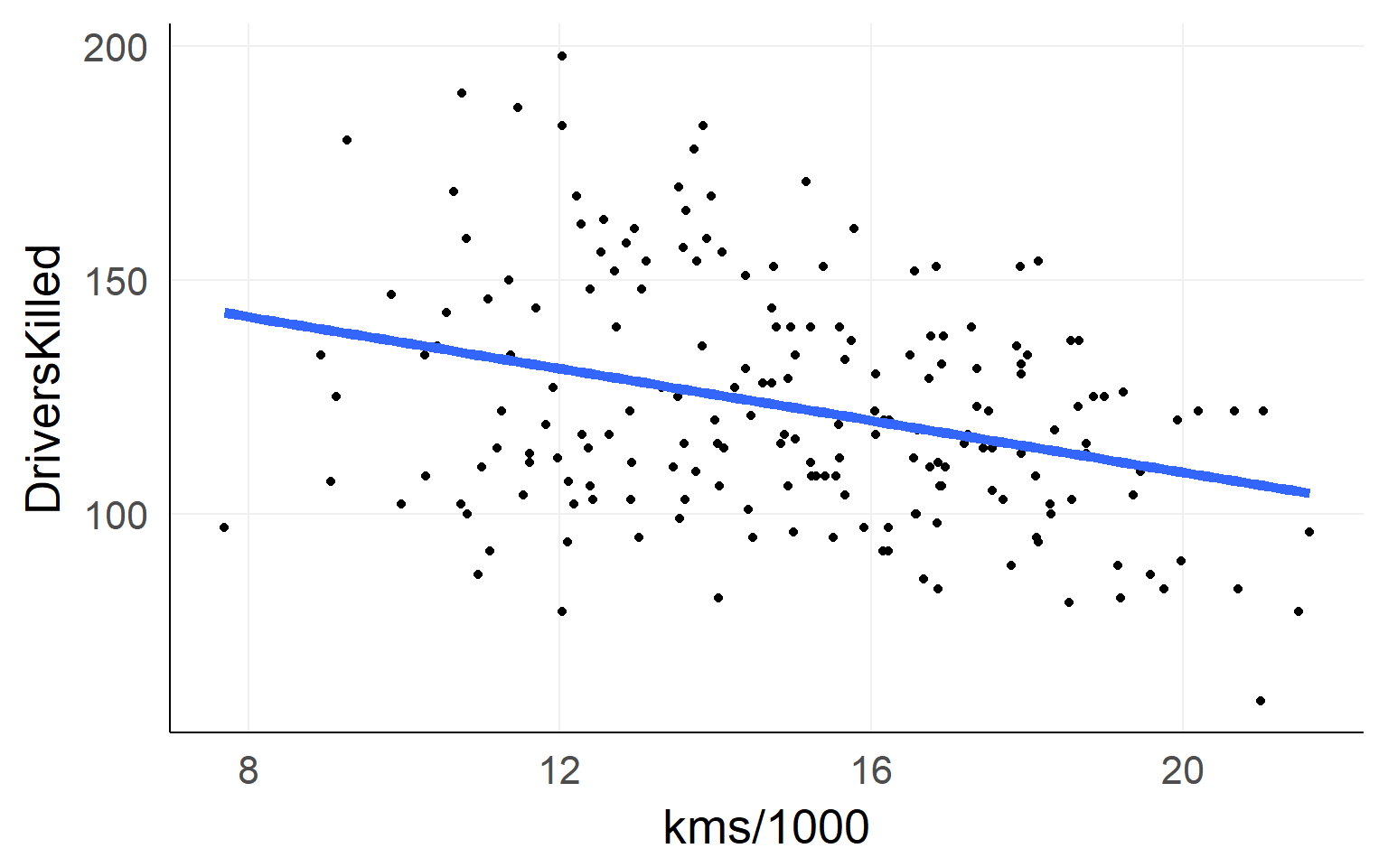
fit = lm(DriversKilled~1+kms,data)Lines are simple! Intercept + Slope
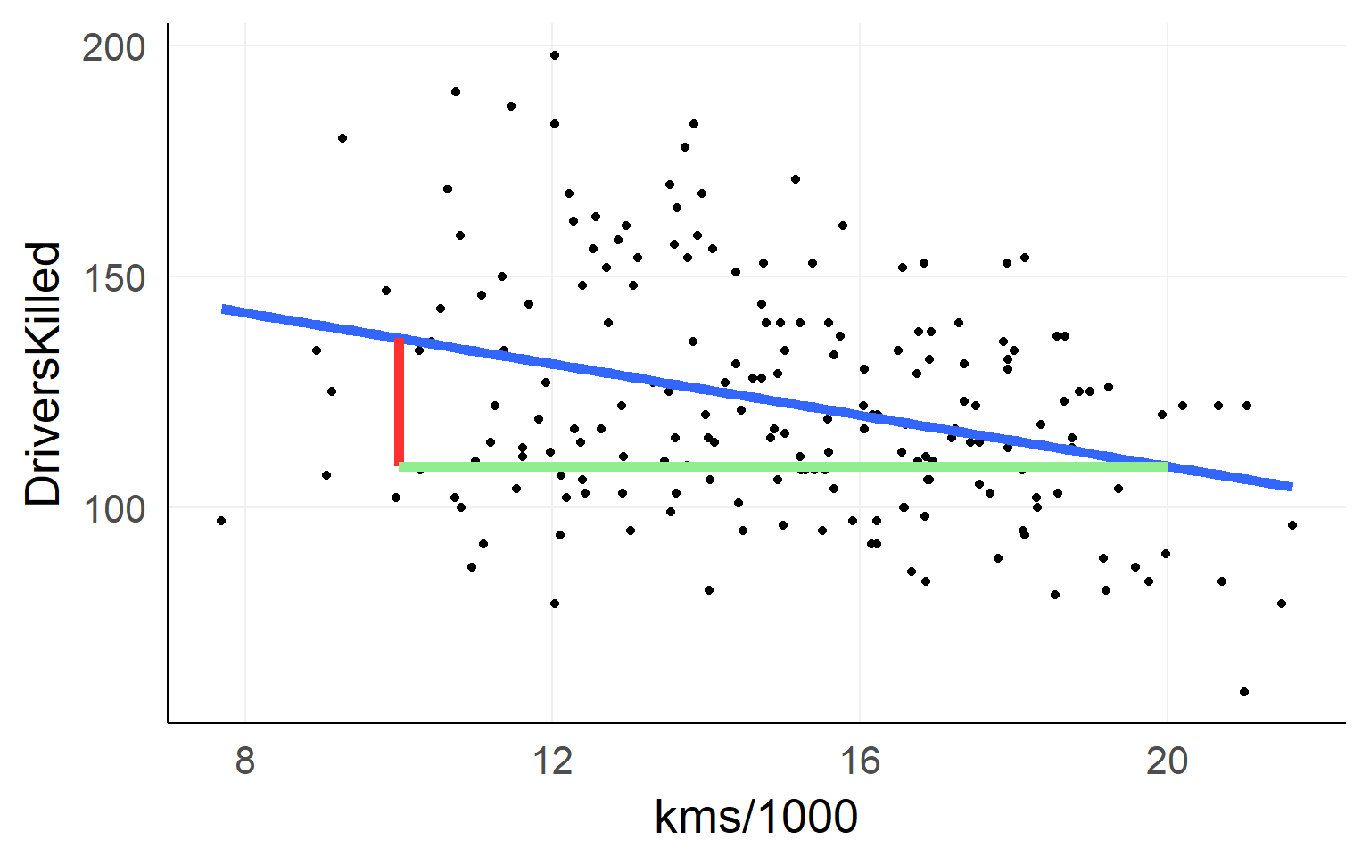
\[ DriversKilled = \beta_0 + (kms/1000) * \beta_1 \]
Red Line: \([DriversKilled | kms/1000==20] - [DriversKilled | kms/1000==10]\)
\(=\beta_0 + 20\beta_1 - (\beta_0 + 10\beta_1)\) \(=10\beta_1\)
Which line to choose?
Residuals / L2 Norm
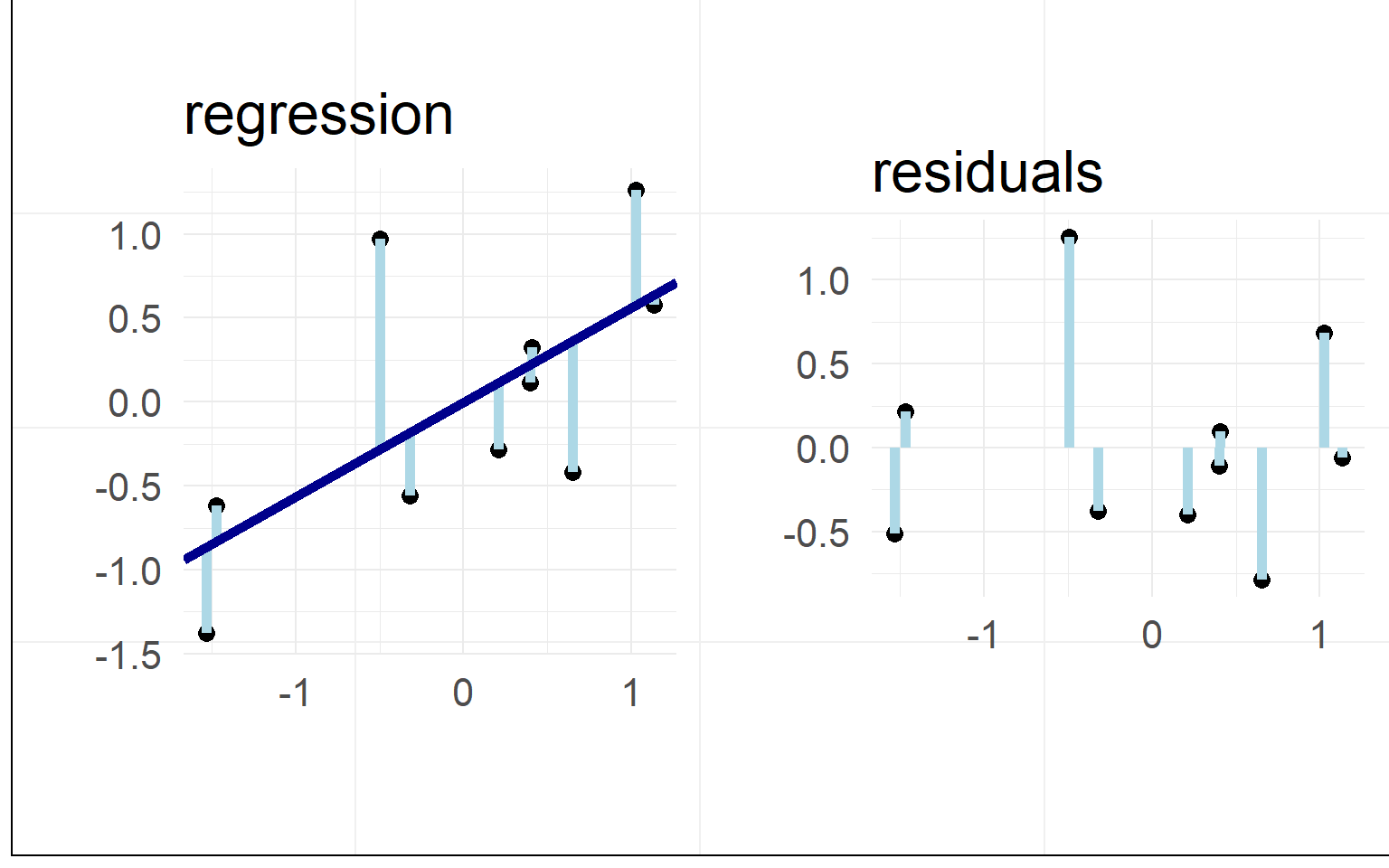
Minimizing the residuals maximizes the fit
L2-Norm (Least Squares): \(min(|residual_i|_2)\)
In our example
Data: \(y = \beta_0 + x_1 \beta_1 + e_i\)
Prediction: \(\hat{y} = \beta_0 + x_1 \beta_1\)
Residuals: \(e_i = y - \hat{y}\)
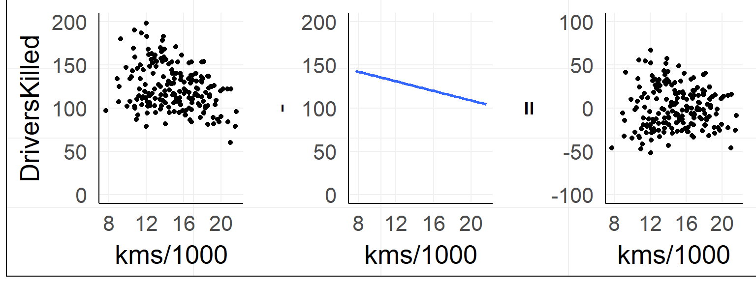
Explained Variance
(I modified the example data for clarity)
Single outlier
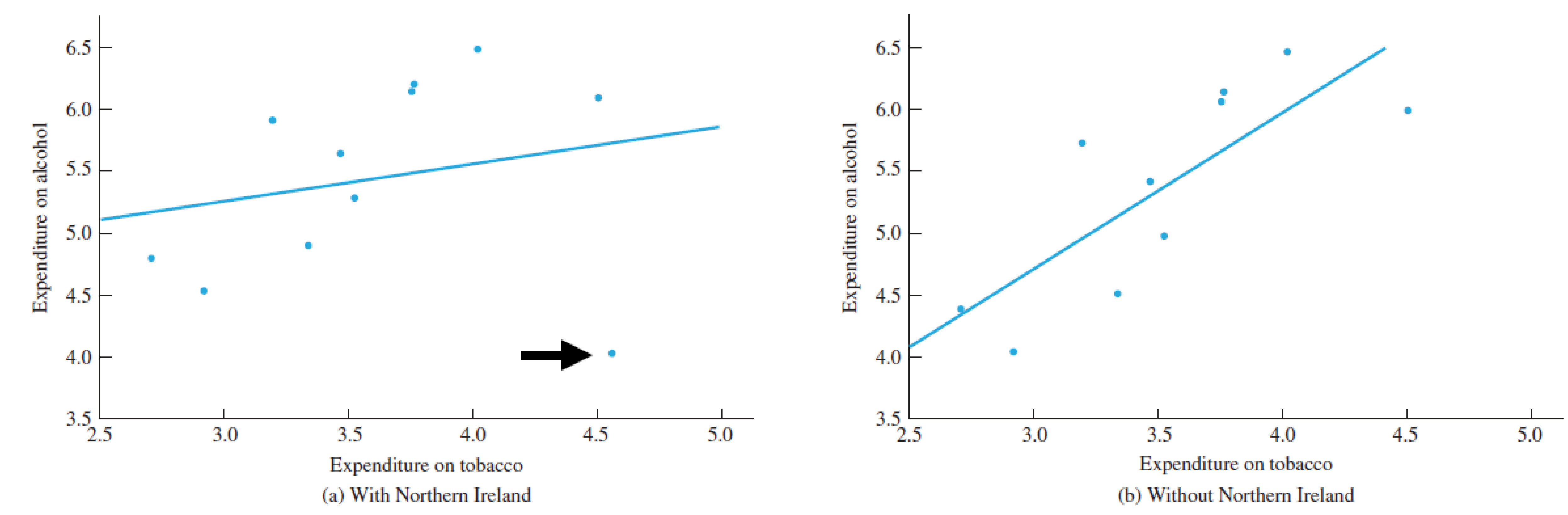 Especially true for small sample sizes
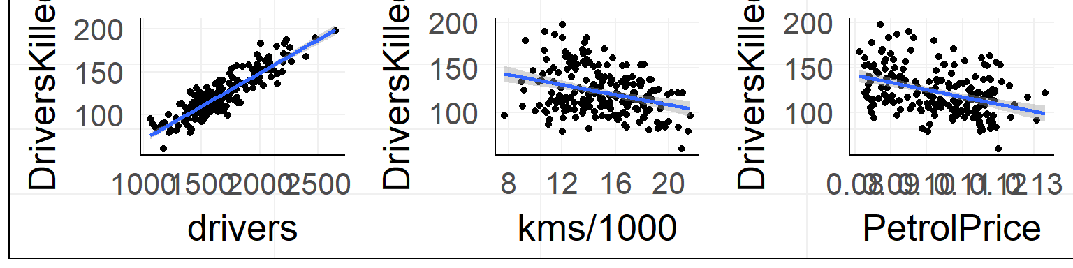
summary(lm(DriversKilled ~ kms + drivers + PetrolPrice,data = data))##
## Call:
## lm(formula = DriversKilled ~ kms + drivers + PetrolPrice, data = data)
##
## Residuals:
## Min 1Q Median 3Q Max
## -27.333 -7.848 -0.532 7.544 35.036
##
## Coefficients:
## Estimate Std. Error t value Pr(>|t|)
## (Intercept) -2.642e+01 1.254e+01 -2.107 0.0365 *
## kms 7.901e-04 3.255e-04 2.428 0.0161 *
## drivers 8.164e-02 3.429e-03 23.810 <2e-16 ***
## PetrolPrice 9.716e+00 7.911e+01 0.123 0.9024
## ---
## Signif. codes: 0 '***' 0.001 '**' 0.01 '*' 0.05 '.' 0.1 ' ' 1
##
## Residual standard error: 11.53 on 188 degrees of freedom
## Multiple R-squared: 0.7969, Adjusted R-squared: 0.7937
## F-statistic: 245.9 on 3 and 188 DF, p-value: < 2.2e-16With two predictors you span a plane
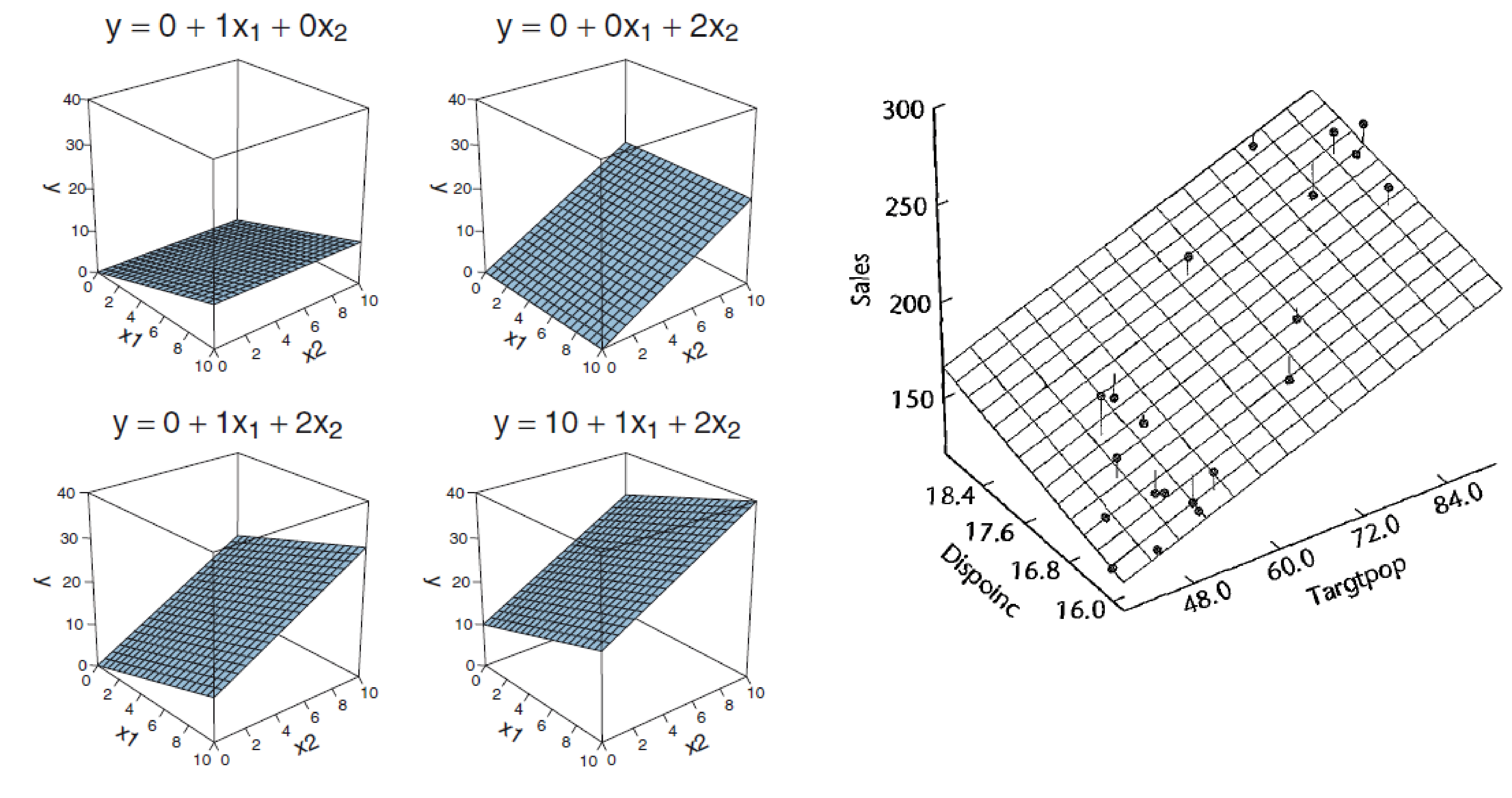
Overlapping variance
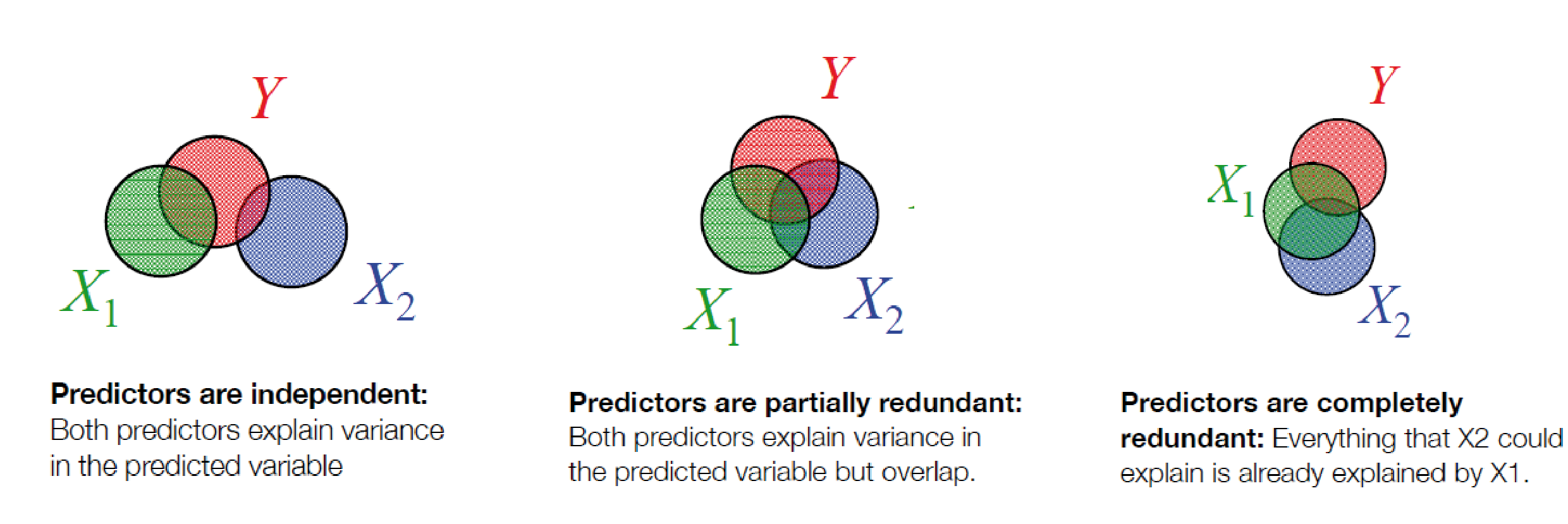
a graphical intuition
Dummy Coding
Dummy Coding
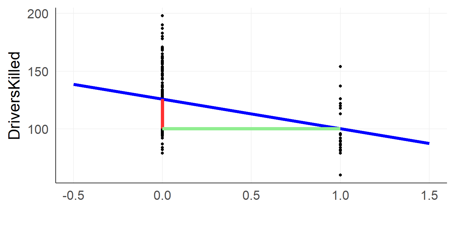
We code the categorical variable with 0 / 1
\(y_i = \beta_0 + is\_law *\beta_1 + e_i\)
Effect Coding aka sum coding aka deviation coding
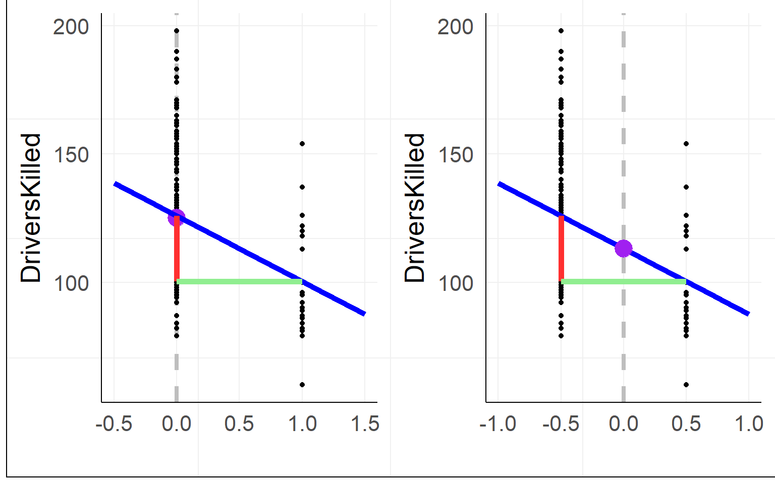
Using effect coding, the interpretation of the intercept changes to the mean between groups
warning: often effect coding is made using -1 and 1, then the \(\beta_1\) is halve the size! using 0.5 is much more practical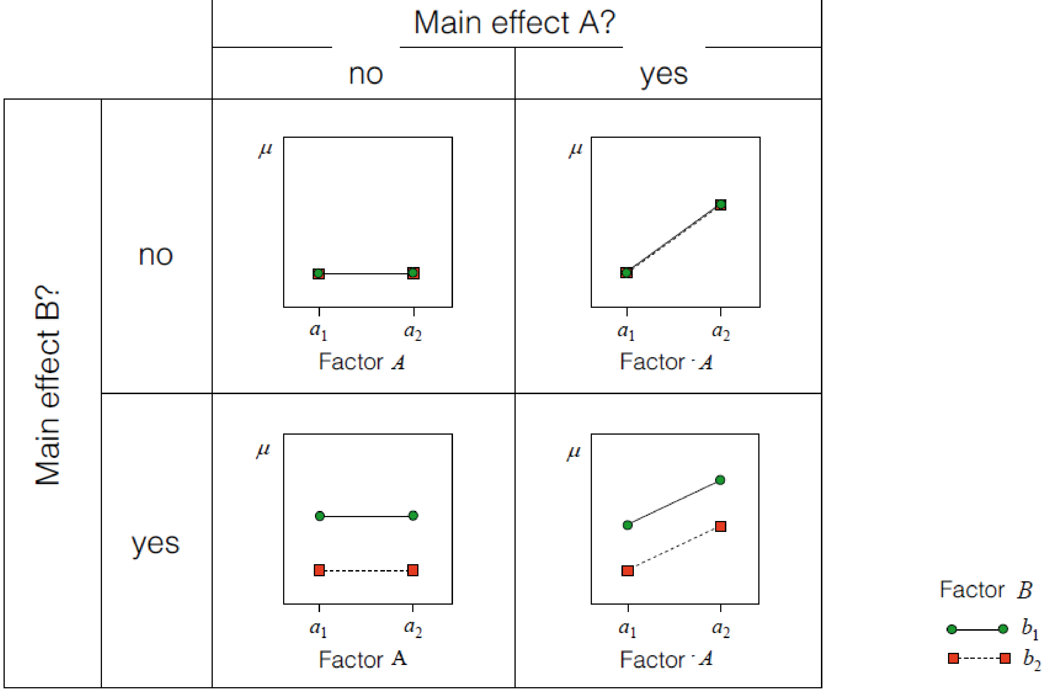 errorbars/data-points ommited for clarity
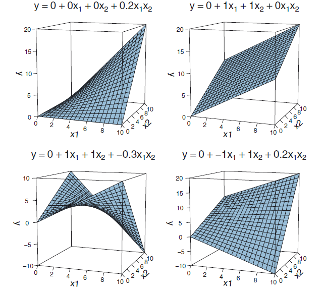
Interaction effects
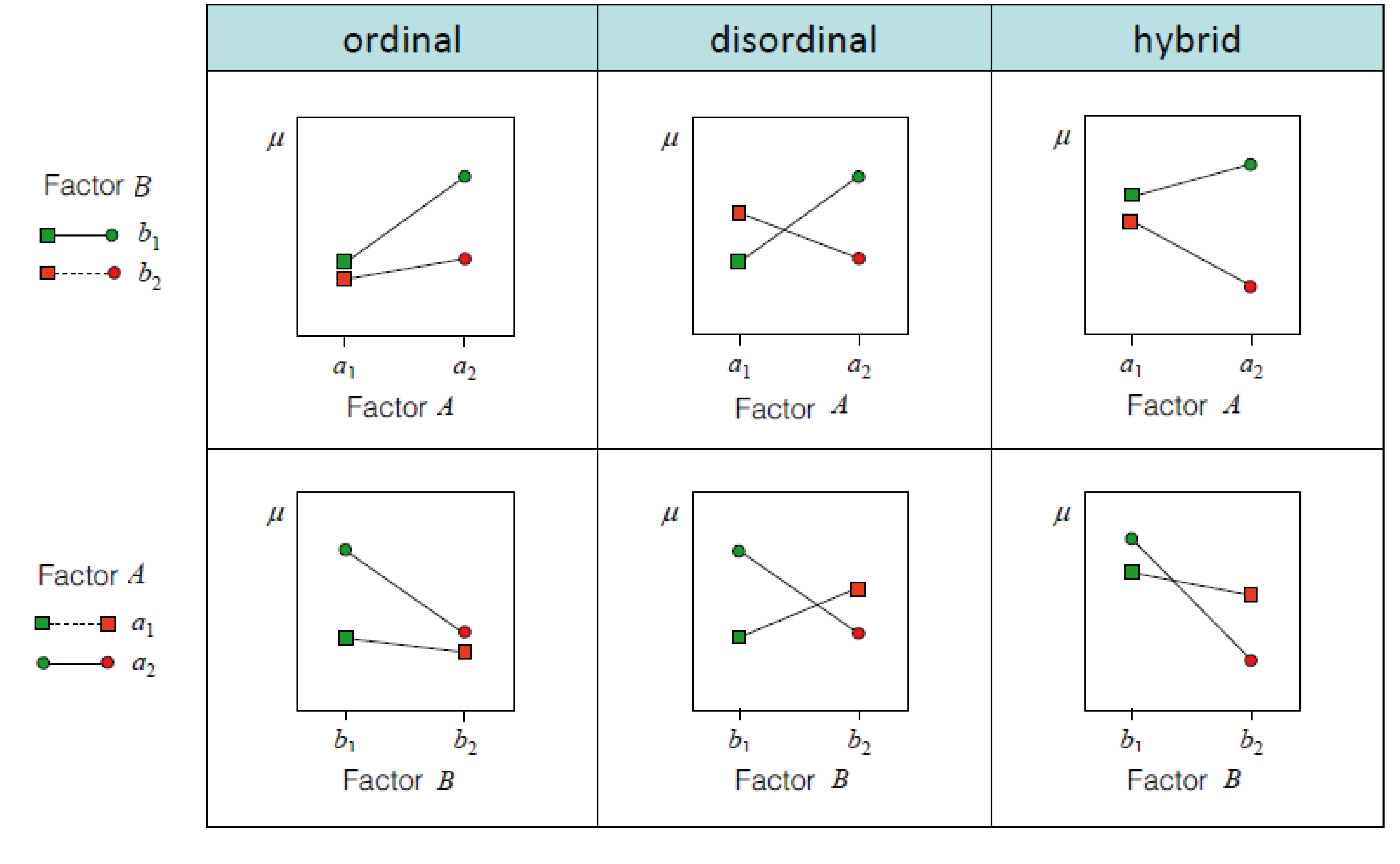
Interactions of continuous/categorical predicotrs
\(y = \beta_0 + factorA * \beta_1 + contB * \beta_2 + factorA * contB * \beta_3\) 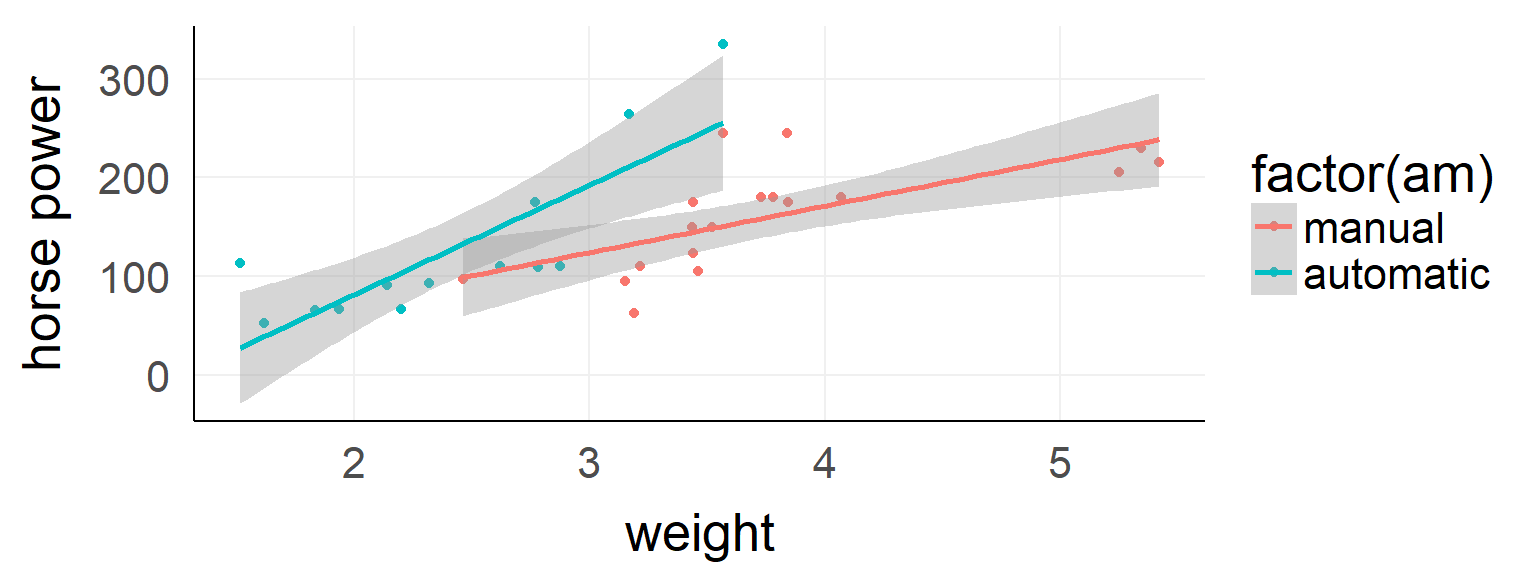
##
## Call: lm(formula = hp ~ wt * am, data = d)
##             Estimate Std. Error t value Pr(>|t|)
## (Intercept)   -17.39      52.44  -0.332  0.74260
## wt             47.14      13.64   3.456  0.00177 **
## am           -123.33      74.03  -1.666  0.10690
## wt:am          63.84      25.08   2.545  0.01672 *
##
## Residual standard error: 44.99 on 28 degrees of freedom
## Multiple R-squared:  0.6111, Adjusted R-squared:  0.5694
## F-statistic: 14.66 on 3 and 28 DF, p-value: < 1e-04The difference between main and simple effects
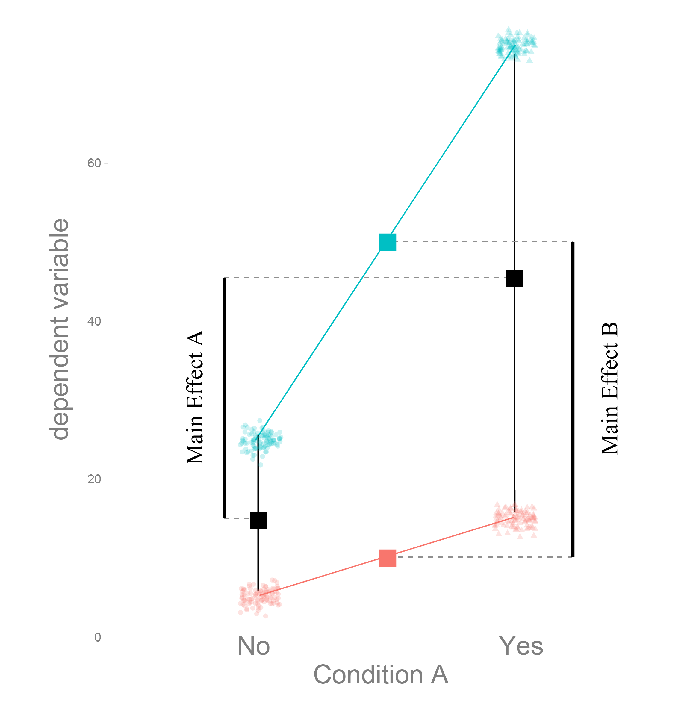
Dummy coding tests simple effects
Effect coding main effects
Interaction between two continuous variables
##
## Call:
## lm(formula = read ~ math * socst, data = dSoc)
##
## Residuals:
##      Min       1Q   Median       3Q      Max
## -18.6071  -4.9228  -0.7195   4.5912  21.8592
##
## Coefficients:
##              Estimate Std. Error t value Pr(>|t|)
## (Intercept) 37.842715  14.545210   2.602  0.00998 **
## math        -0.110512   0.291634  -0.379  0.70514
## socst       -0.220044   0.271754  -0.810  0.41908
## math:socst   0.011281   0.005229   2.157  0.03221 *
## ---
## Signif. codes:  0 '***' 0.001 '**' 0.01 '*' 0.05 '.' 0.1 ' ' 1
##
## Residual standard error: 6.96 on 196 degrees of freedom
## Multiple R-squared:  0.5461, Adjusted R-squared:  0.5392
## F-statistic: 78.61 on 3 and 196 DF,  p-value: < 2.2e-16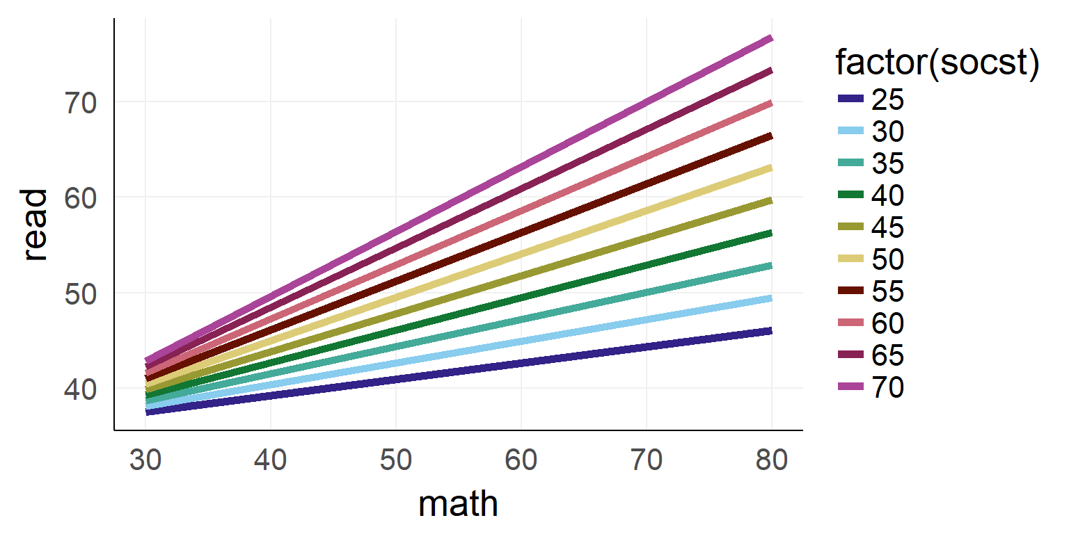
Interaction as a plane
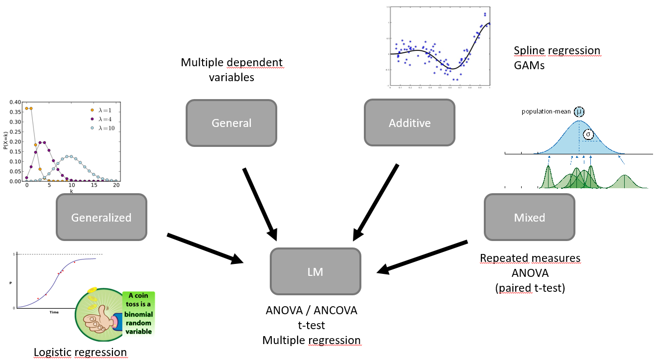
Remember: There is only one statistical test
We need to specify our H0
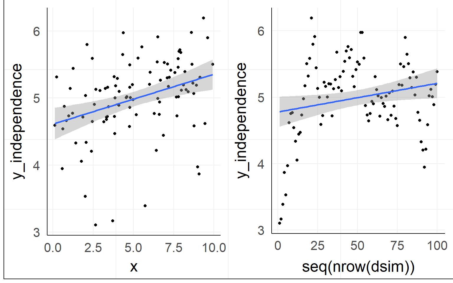
General assumption for all of the following inference: Independence of residuals
What is a standard error?
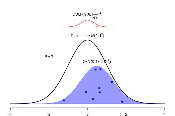
\(SEM = \frac \sigma{\sqrt{N}}\)
Confidence Interval as an area of the sampling distribution
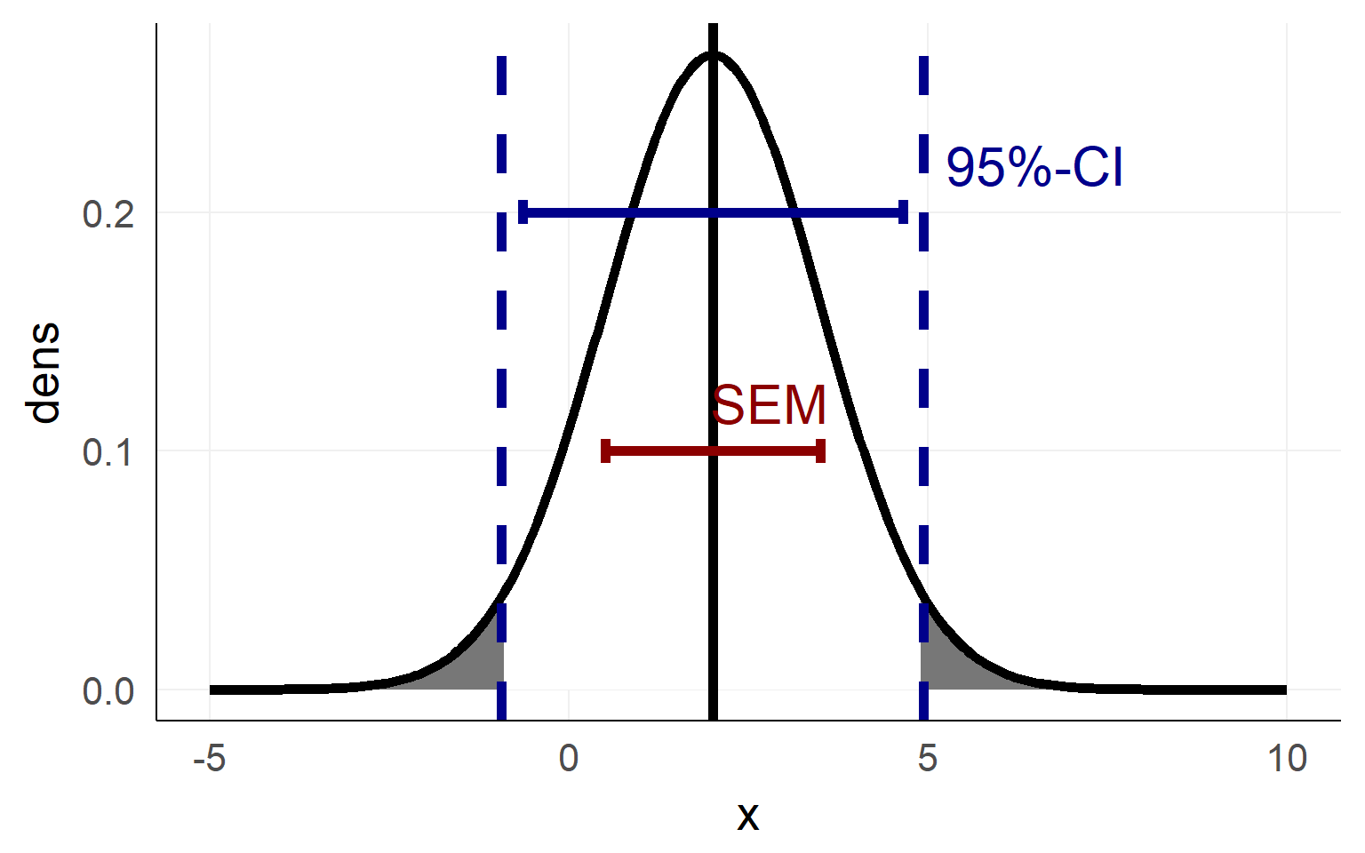
Just to be sure: Mr. Mean

What is a t-distribution?
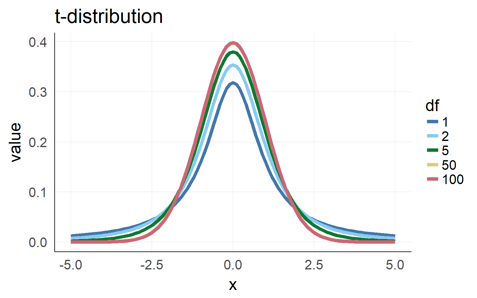
Population \(\sigma\) is unknown. Sampling \(\hat \sigma\) has to be used.
=> Sampling distribution (for small n) is not normal distributed but student t-distributed (with given degrees of freedom)
Empirical distribution:
Analytic solution
An analytical form is available here as well
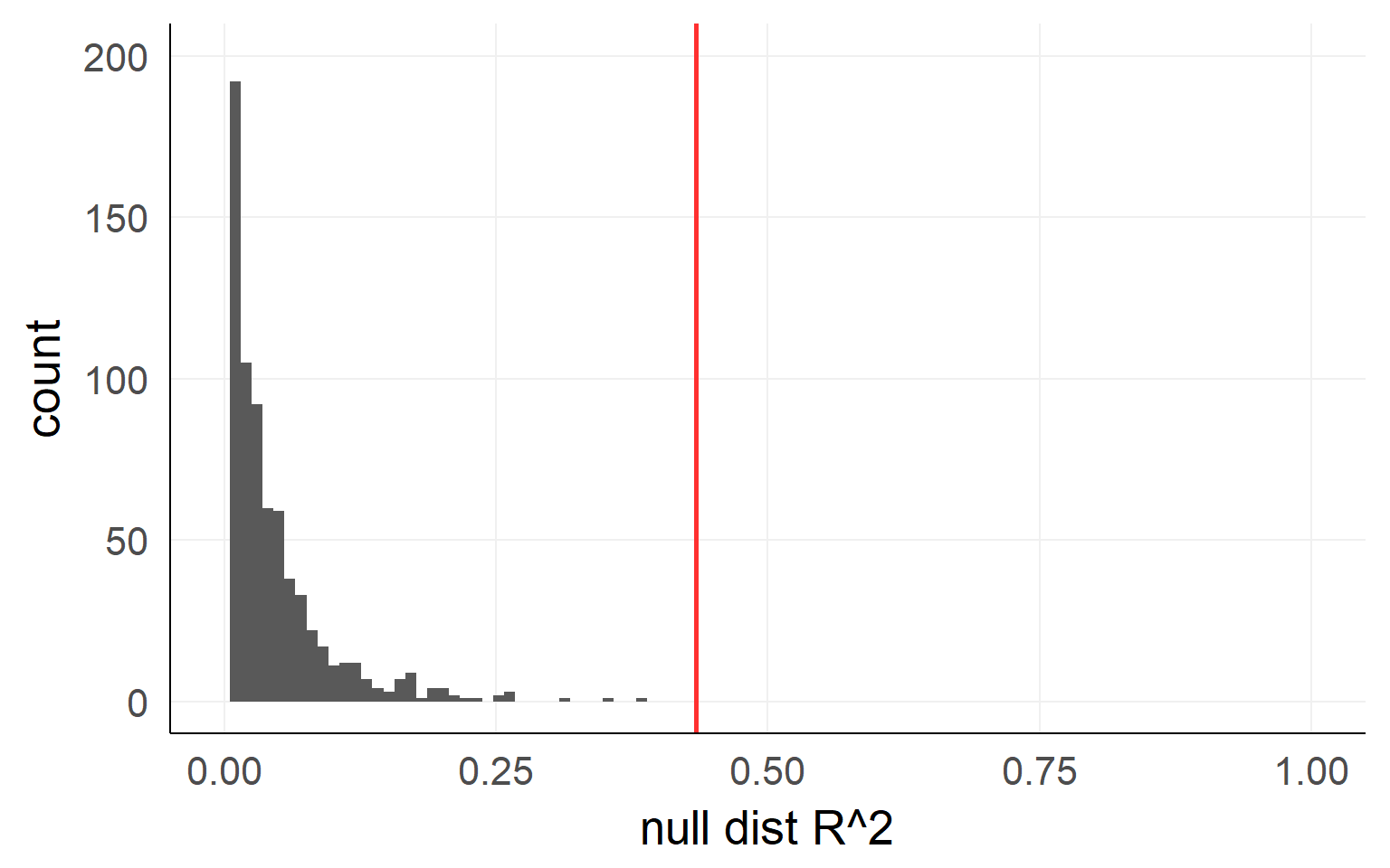
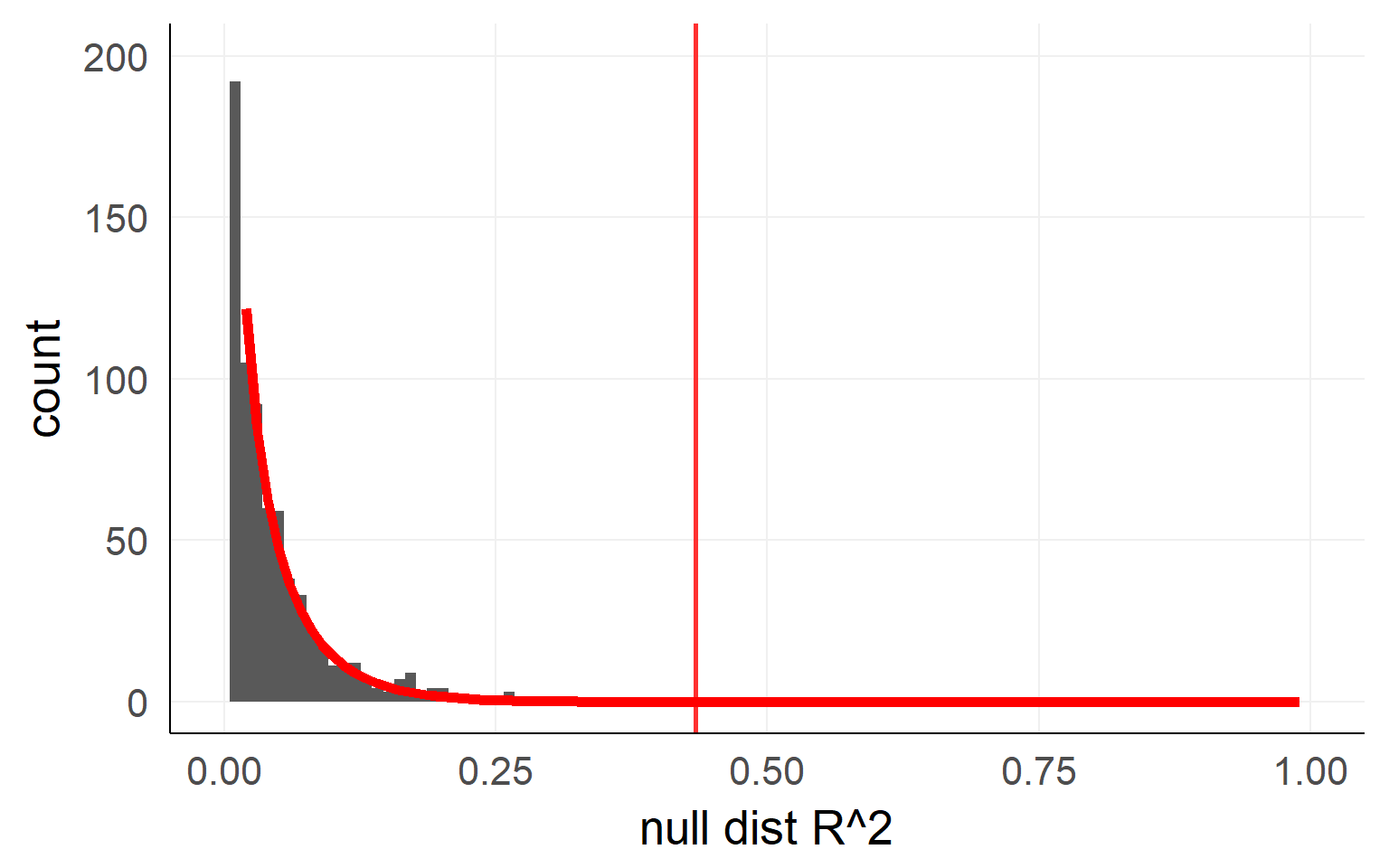
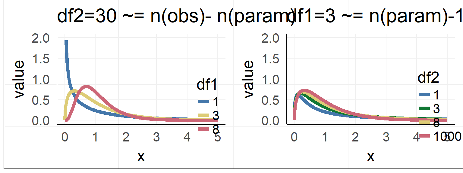
Usually F-distribution is used
\[ F = \frac{\frac{R^2_{m+k}-R^2_{m}}{df_1}}{\frac{1-R^2_{m+k}}{df_2}} = \frac{R^2_{m+k}-R^2_{m}}{1-R^2_{m+k}} * \frac{df_2}{df_1}\] with bookkeeping (for 1xk ANOVA):
\(df_1 = k\), with \(k\) the number of predictors
\(df_2 = n - m - k -1\), with \(n\) the number of observations, \(m\) the number of total predictors
Overfit
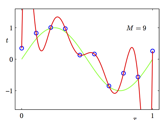
var-explained(predictorA) \(<=\) Var-explained(predictorA + predictorB)
Explained-variance is not everything. We also have to take into account the number of predictors we include
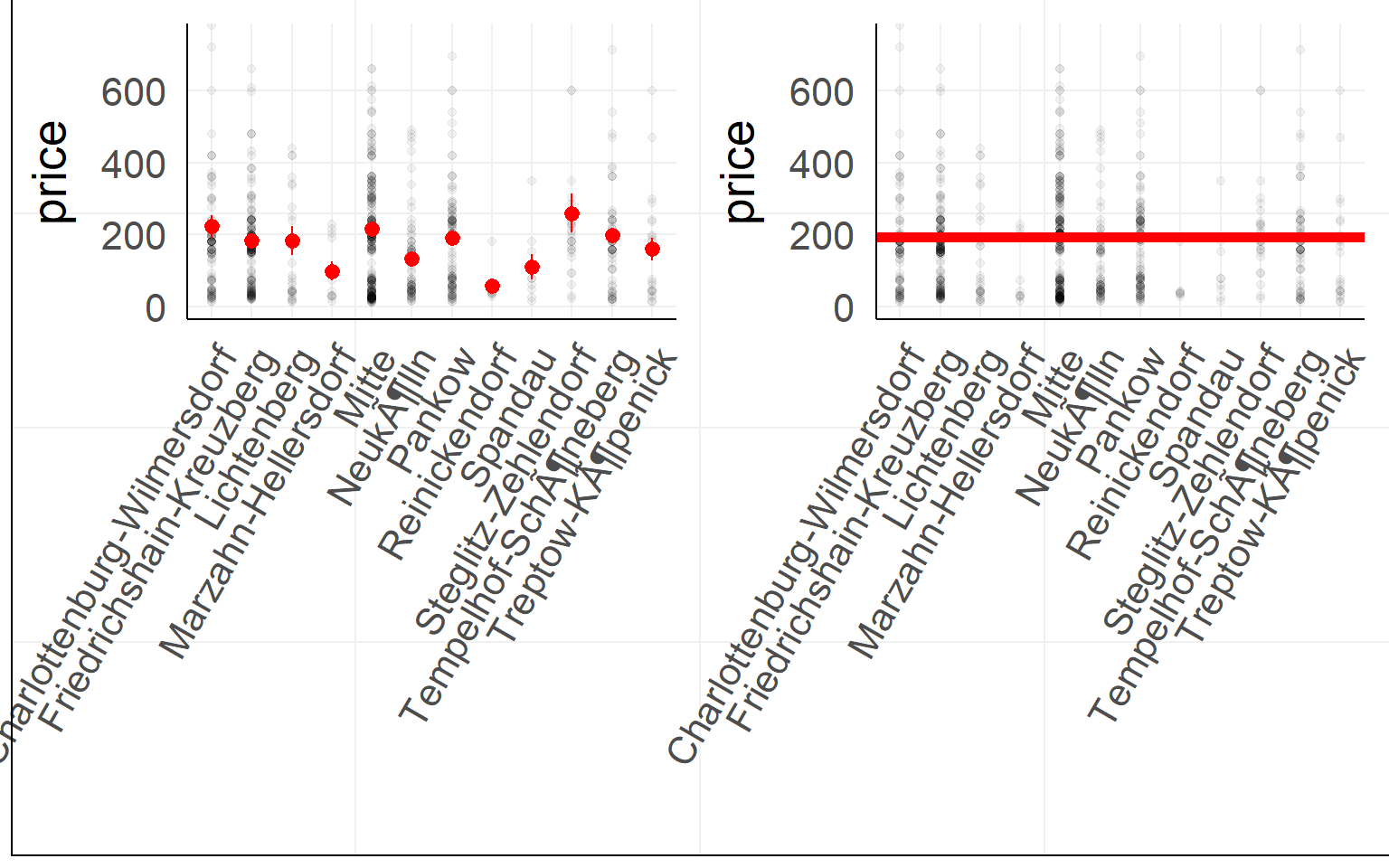
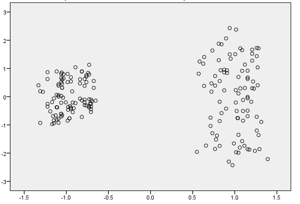
Categorical predictor with multiple levels
Airbnb prices against location in Berlin (first 900 entries)
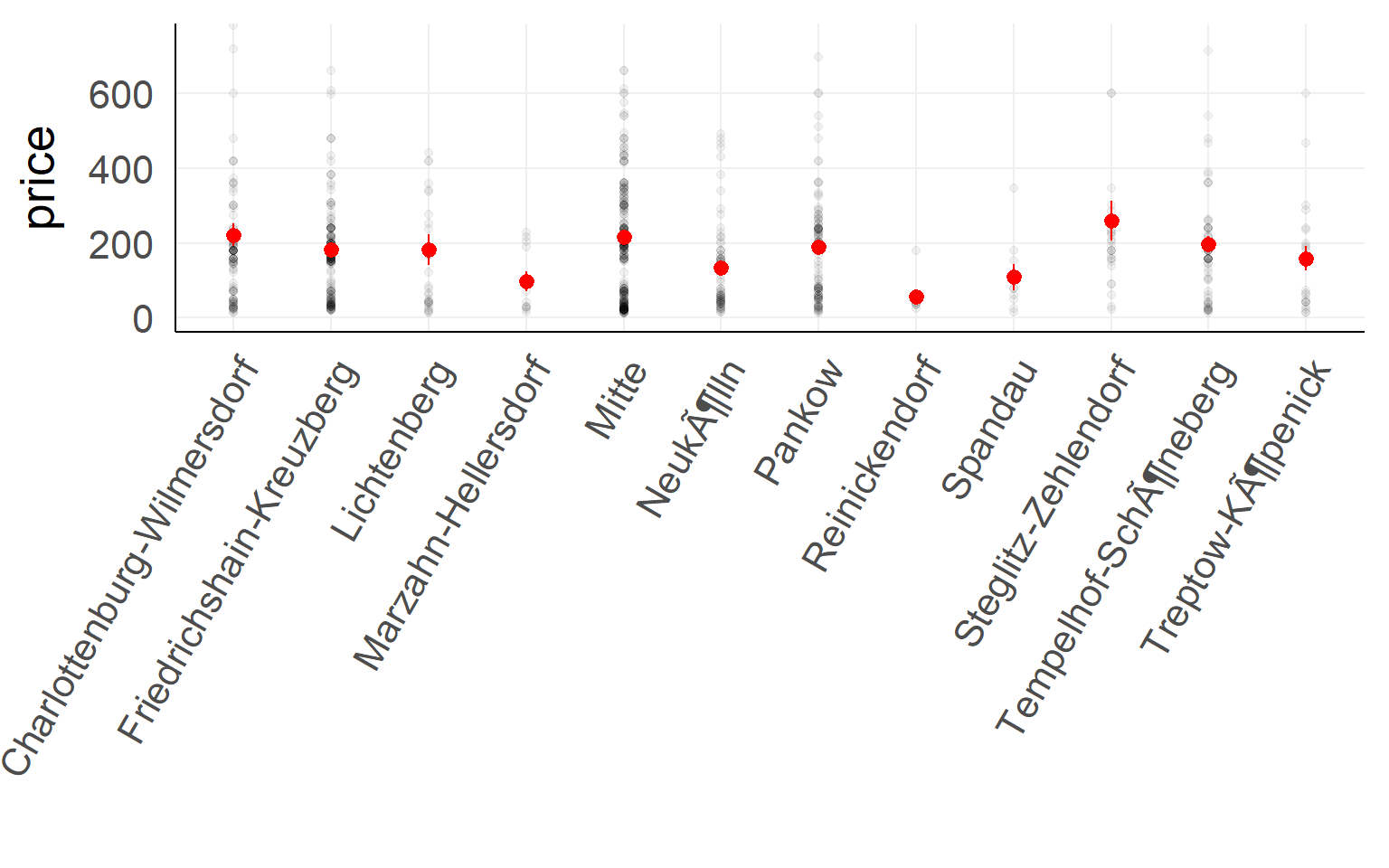
Testing
summary(lm(price~1+ngb,dair[1:900,]))##
## Call:
## lm(formula = price ~ 1 + ngb, data = dair[1:900, ])
##
## Residuals:
## Min 1Q Median 3Q Max
## -237.30 -134.55 -27.47 45.21 2822.60
##
## Coefficients:
## Estimate Std. Error t value Pr(>|t|)
## (Intercept) 222.113 22.833 9.728 <2e-16 ***
## ngbFriedrichshain-Kreuzberg -38.717 28.353 -1.366 0.1724
## ngbLichtenberg -39.647 46.980 -0.844 0.3989
## ngbMarzahn-Hellersdorf -124.022 71.546 -1.733 0.0834 .
## ngbMitte -6.562 26.621 -0.246 0.8054
## ngbNeukölln -89.534 35.416 -2.528 0.0116 *
## ngbPankow -32.324 31.064 -1.041 0.2984
## ngbReinickendorf -166.256 88.011 -1.889 0.0592 .
## ngbSpandau -112.891 78.361 -1.441 0.1500
## ngbSteglitz-Zehlendorf 37.183 48.933 0.760 0.4475
## ngbTempelhof-Schöneberg -24.770 36.215 -0.684 0.4942
## ngbTreptow-Köpenick -62.896 52.155 -1.206 0.2282
## ---
## Signif. codes: 0 '***' 0.001 '**' 0.01 '*' 0.05 '.' 0.1 ' ' 1
##
## Residual standard error: 224.9 on 888 degrees of freedom
## Multiple R-squared: 0.02032, Adjusted R-squared: 0.008188
## F-statistic: 1.675 on 11 and 888 DF, p-value: 0.07433
an graphical way to think about it
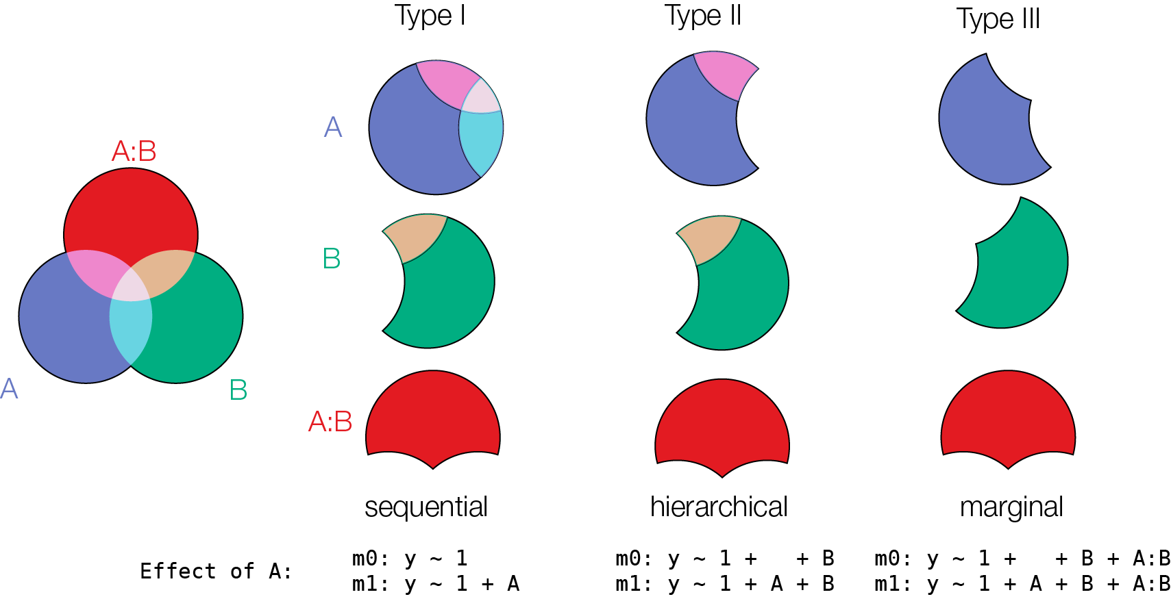
Coming back to a 2x2 design. Which order to test effects?
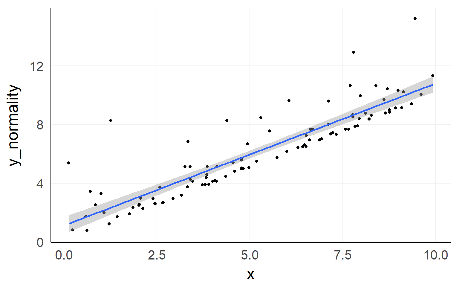
Linearity of responses
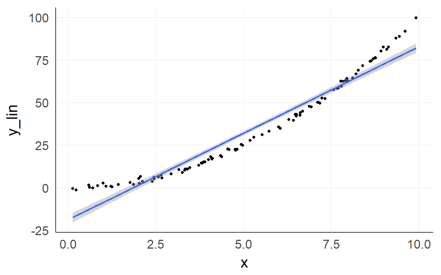
Linear response
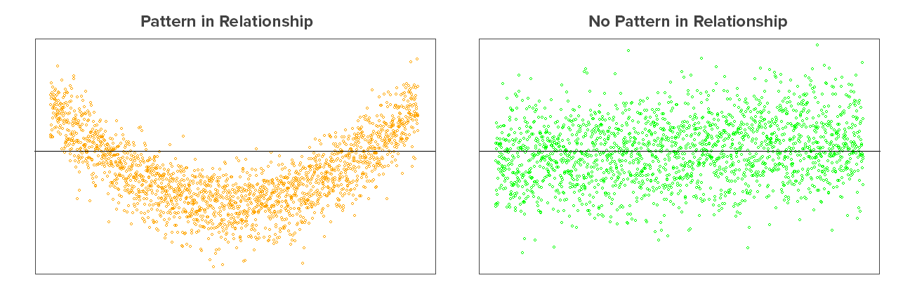
Independence of residuals
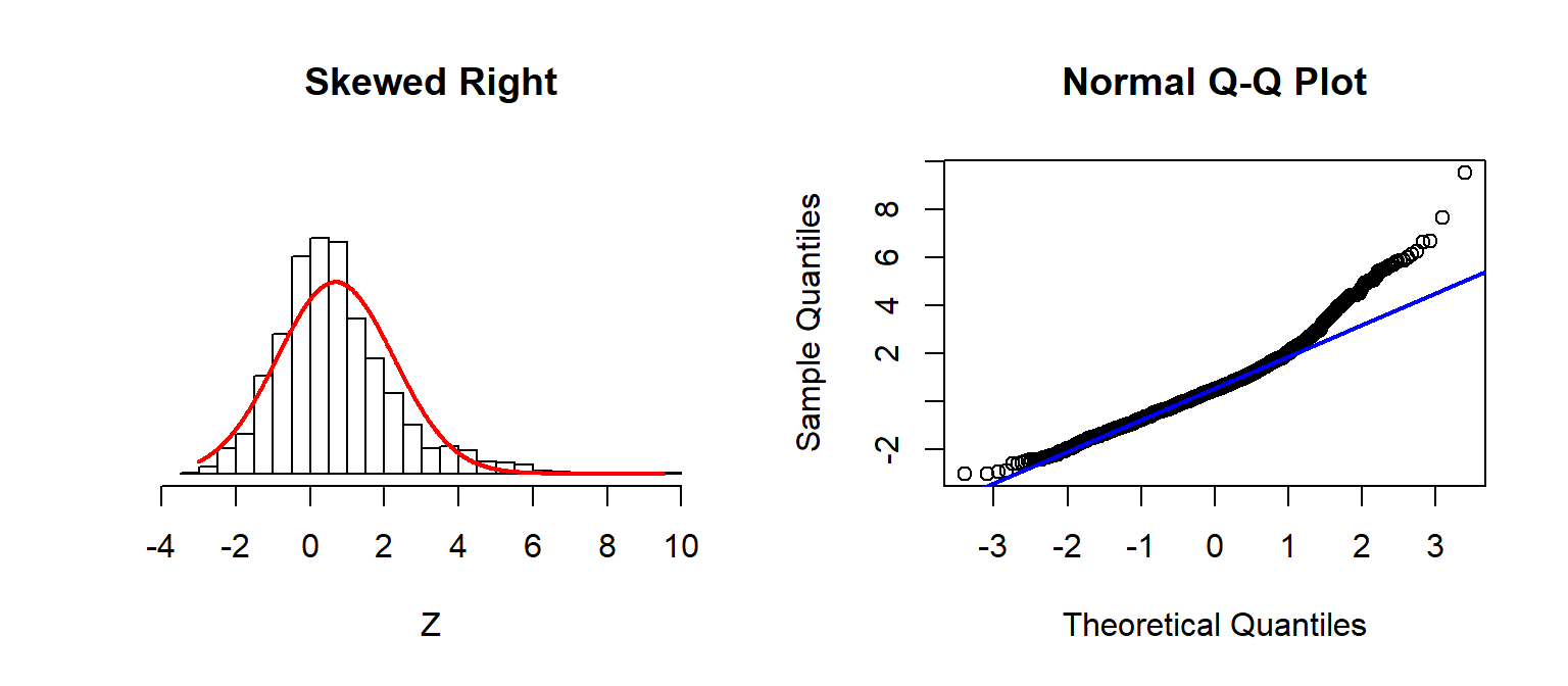
Normality of residuals
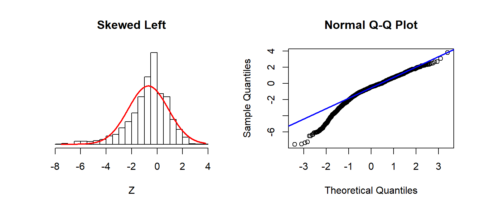
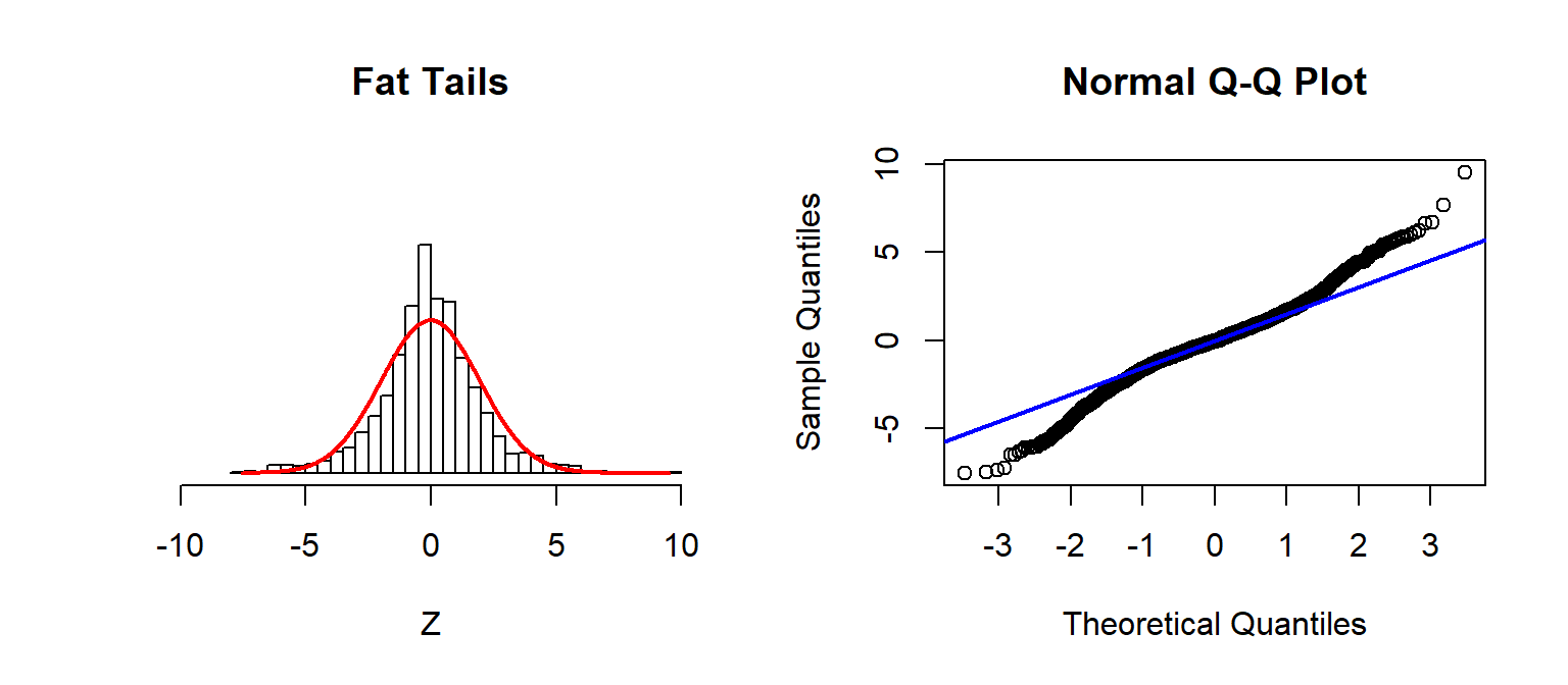
Checking Assumptions: Normality using QQplots
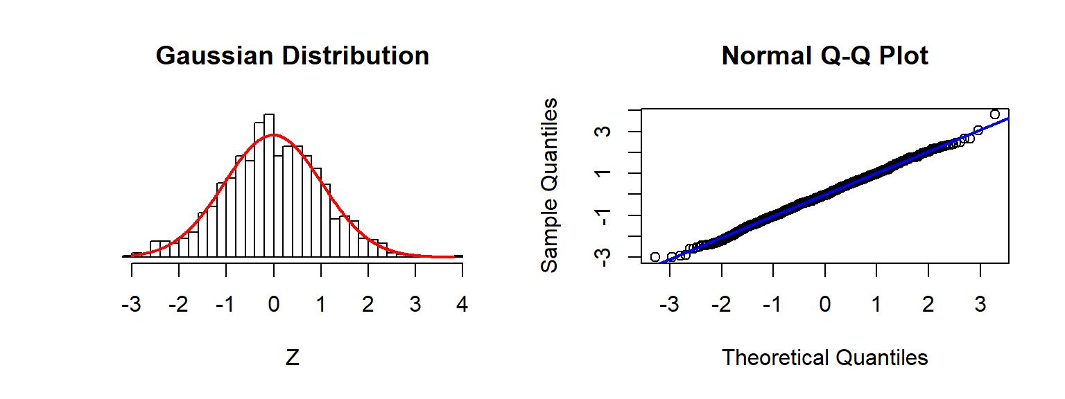
Source: Sean Kross
A nice trick
simulate datasets with same specifications and compare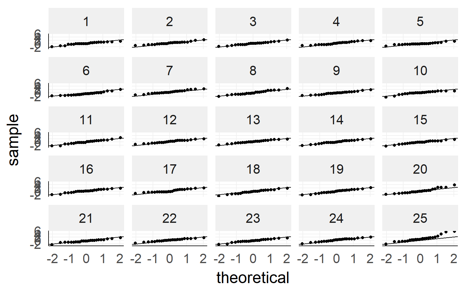
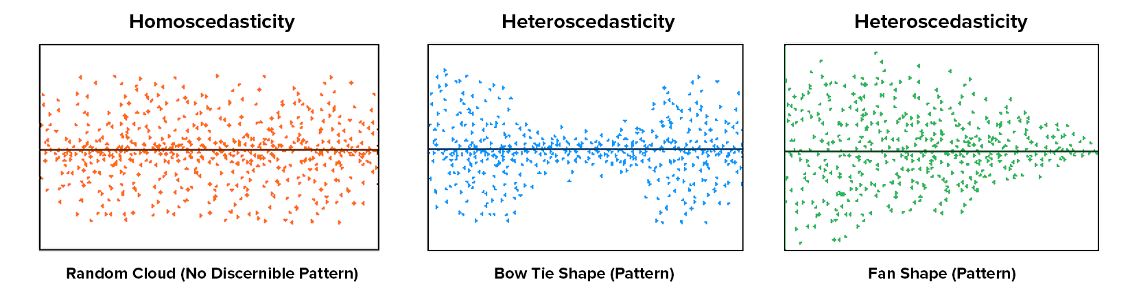
Equal variance
Bootstrapping in R
##
## Call: lm(formula = read ~ math * socst, data = dSoc)
##              Estimate Std. Error t value Pr(>|t|)
## (Intercept) 37.842715  14.545210   2.602  0.00998 **
## math        -0.110512   0.291634  -0.379  0.70514
## socst       -0.220044   0.271754  -0.810  0.41908
## math:socst   0.011281   0.005229   2.157  0.03221 *
##
## Residual standard error: 6.96 on 196 degrees of freedom
## Multiple R-squared:  0.5461, Adjusted R-squared:  0.5392
## F-statistic: 78.61 on 3 and 196 DF,  p-value: < 1e-04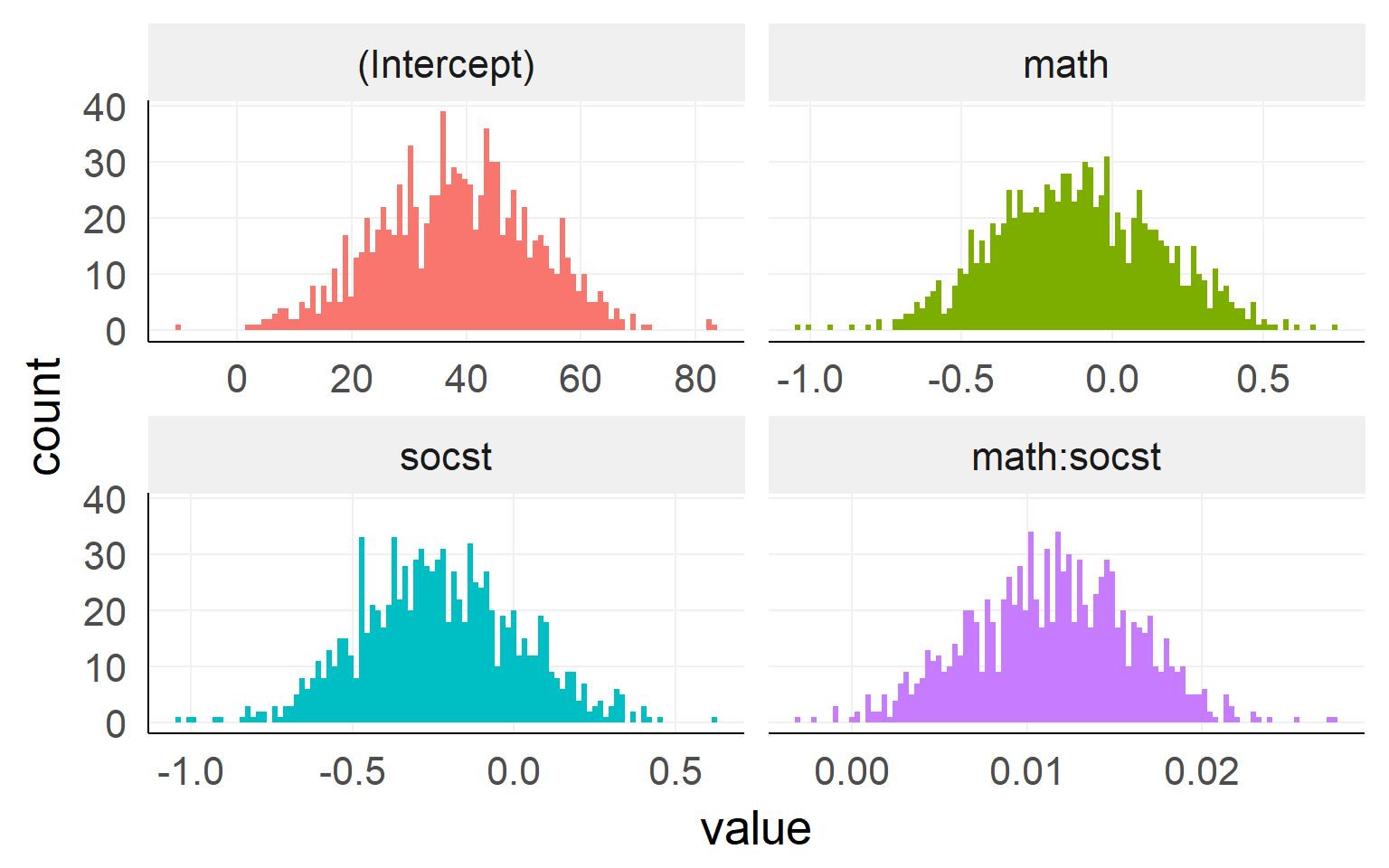
Type I vs. Type II errors
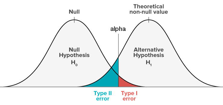
Type Errors
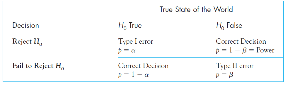
Be both if you can!
Come join our Seminar: “Statistical Rethinking Reading Club” next semester
“This is a rare and valuable book that combines readable explanations, computer code, and active learning.” —Andrew Gelman, Columbia University
“…an impressive book that I do not hesitate recommending for prospective data analysts and applied statisticians!” —Christian Robert, Université Paris-Dauphine (review)
“A pedagogical masterpiece…” —Rasmus Bååth, Lund University
“The content of this book has been developed over a decade+ of McElreath’s teaching and mentoring of graduate students, post docs, and other colleagues, and it really shows.” —Brian Wood, Yale
“…omg suddenly everything makes sense…” —Ecstatic anonymous reader
And thats it!