Simulating EEG/ERP Data with SEREEGA & multiple comparison corrections

For the $i^2 c^2 s^3$ summer school I simulated quite a bit of data and analyzed them with several common multiple comparison methods. I used the SEREEGA toolbox for the simulation. All the MatLab-code can be found at the end of this post. In a follow-up blogpost I will extend the toolbox to continuous data that we can analyze with the unfold toolbox.

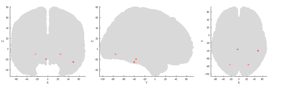
First, I simulated data based on three effects: Two early dipoles representing the P100, one right lateralized for the N170 and a deep one for the P300.

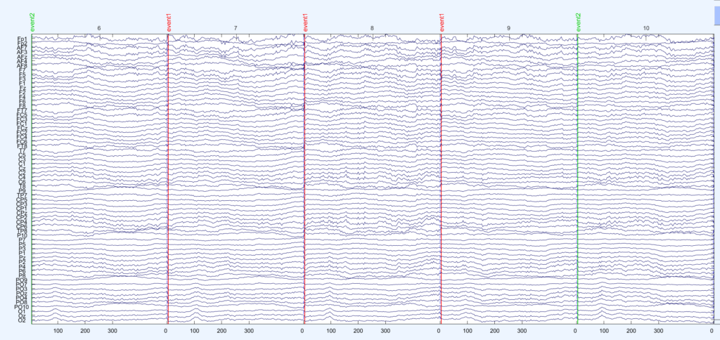
I added brown and white noise to the simulated epochs. An exemplary eegplot shows that it kind of looks like EEG data.

I generate two conditions with two different condition-differences, one on the N170 and one on the P300 . The same data are depicted in the following three plots:

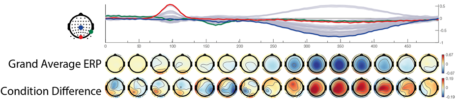
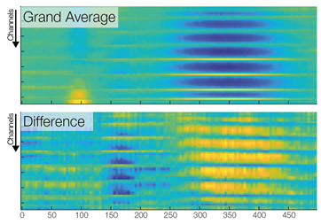
In the first row we see a butterfly plot of activation in all channels (the colored channels are depicted in the next plot). In the first topoplot-row we have the average activation and in the last row we have the condition differences.

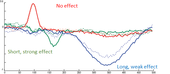
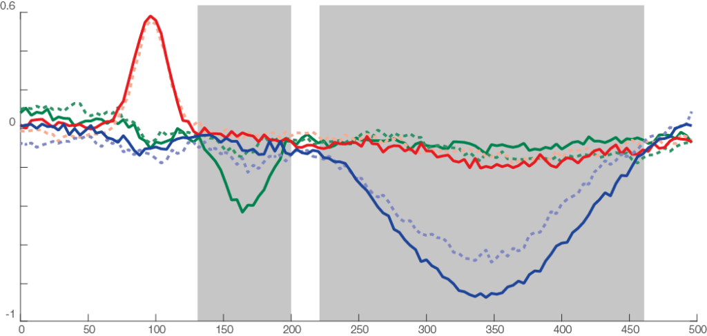
The red line is the P100, occipital effect. No difference between conditions. The green one is the N170, temporal effect. Only visible in one condition. The blue one is a P300 like, deep effect. Difference in amplitude between conditions.

Now we are ready to do some statistical testing and multiple comparison correction. I choose to compare uncorrected, bonferroni-holms, FDR (Benjamini-Hochberg), clustermass cluster permutation testing (LIMO toolbox) and threshold free cluster enhancement (EPT-TFCE toolbox).

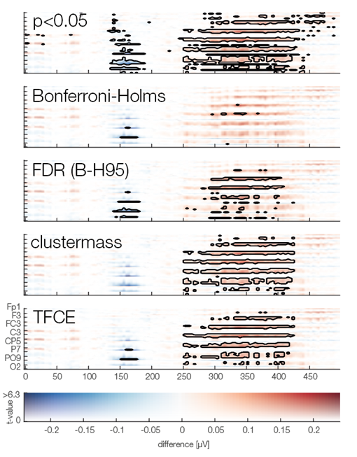
In this instance, uncorrected p-value did not so bad, Bonferroni-Holms is, as expected, quite conservative. FDR hat troubles with the elongated cluster and TFCE/Cluster-permutation with the short one.

Note: This is only a single simulation. In order to move from these anectotal findings to proper statements, one would need to repeat the simulation 1000 times and see how often which samples were deemed significant (see Groppe 2011).

Thanks to Anna Lisa Gert for help with writing this post.

This is the code I used, it is a bit messy because it was programmed in a tutorial-style and I kept my debug-statements in there.

rng(1)
%% Adding toolboxes
addpath('lib\eeglab\')
if ~exist('pop_loadset')
    eeglab
end
addpath(genpath('lib\sereega'))
addpath(genpath('lib\eegvis'))
% Threshold Free cluster enhancement
addpath(genpath('lib\unfold\lib\ept_TFCE'))
addpath(genpath('lib\limo_eeg'))
%% SEREEGA Data Generation
cfg = struct('debug',0)
%% load headmodel 
lf = lf_generate_fromnyhead('montage', 'S64');

if cfg.debug
    plot_headmodel(lf);
end

%% set seed

%% noise
noise_brown = struct( ...
    'type', 'noise', ...
    'color', 'brown', ...
    'amplitude', 2);
noise_brown = utl_check_class(noise_brown);

noise_white = struct( ...
    'type', 'noise', ...
    'color', 'white', ...
    'amplitude', 2);
noise_white = utl_check_class(noise_white);


%% visual Cortex N170
vis = [];

vis.signal{1} = struct();
vis.signal{1}.peakLatency = 170;      % in ms, starting at the start of the epoch
vis.signal{1}.peakWidth = 100;        % in ms
vis.signal{1}.peakAmplitude = -5;      % in microvolt
vis.signal{1} = utl_check_class(vis.signal{1}, 'type', 'erp');
vis.signal{2} = noise_brown;


% right visual cortex
vis.source= lf_get_source_nearest(lf, [50 -40 -25]);
if cfg.debug
    plot_source_location(vis.source, lf, 'mode', '3d','shrink',0);
end

% vis.orientation = utl_get_orientation_pseudotangential(vis.source,lf); 
vis.orientationDv = [0 0 0]; % orientation does not change between trials
vis.orientation = [0.5,-0.46,1]; % I looked at the maps and found that this prientation most closely looked like a N170

if cfg.debug
    %% This Code I used to generate random orientations and inspect the leadfield projections
    for k = 1:10
        vis.orientation = utl_get_orientation_random(1)
        plot_source_projection(vis.source, lf, 'orientation', vis.orientation,'orientedonly',1);
        %     title(vis.orientation)
    end
end
%% Generate P100, take from SEREEGA Toolbox
p100 = utl_get_component_fromtemplate('visual_p100_erp',lf);
if cfg.debug
    % Visualize the response 
    plot_signal_fromclass(vis.signal{1}, epochs);
end

%% Generate P300
p3 = [];

p3.signal{1} = struct();
p3.signal{1}.peakLatency = 350;      % in ms, starting at the start of the epoch
p3.signal{1}.peakWidth = 400;        % in ms
p3.signal{1}.peakAmplitude = -3;      % in microvolt
p3.signal{1} = utl_check_class(p3.signal{1}, 'type', 'erp');
p3.signal{2} = noise_brown;


% somewhere deep in the brain
p3.source= lf_get_source_nearest(lf, [0 -40 -25]);
if cfg.debug
    %% visualize it using SEREEGA
    plot_source_location(p3.source, lf, 'mode', '3d');
end

p3.orientation = utl_get_orientation_pseudotangential(p3.source,lf);
p3.orientationDv = [0 0 0];

p3.orientation = [0.03,-0.16,1];
if cfg.debug
    %% again find an orientation that somehow matches P300topography
    for k = 1:10
        p3.orientation = utl_get_orientation_random(1)
        plot_source_projection(p3.source, lf, 'orientation', p3.orientation,'orientedonly',1);
    end
end


%% generate 25 random noise sources and combine all components
sources = lf_get_source_spaced(lf, 10, 25);
noise_brown.amplitude = 5;
comps = utl_create_component(sources, noise_brown, lf);
comps = utl_add_signal_tocomponent(noise_white,comps);
[comps1, comps2] = deal(comps);

% add P100 to noise components
comps1(end+1:end+2) = p100; %bilateral
comps2(end+1:end+2) = p100;

% N170 with condition difference
vis.signal{1}.peakAmplitude = -3;
comps1(end+1) = vis;
vis.signal{1}.peakAmplitude = -1;
comps2(end+1) = vis;

% broad, weak P300, with condition difference
p3.signal{1}.peakAmplitude = -10;
comps1(end+1) = p3;
p3.signal{1}.peakAmplitude = -12;
comps2(end+1) = p3;
%% Generate The EEG Data
epochs = struct();
epochs.n = 50;             % the number of epochs to simulate
epochs.srate = 250;        % their sampling rate in Hz
epochs.length = 500;

data1 = generate_scalpdata(comps1, lf, epochs);
data2 = generate_scalpdata(comps2, lf, epochs);
EEG1 = utl_create_eeglabdataset(data1, epochs, lf, 'marker', 'event1');
EEG2 = utl_create_eeglabdataset(data2, epochs, lf, 'marker', 'event2');
EEG = utl_reorder_eeglabdataset(pop_mergeset(EEG1, EEG2));

%% First inspection, this should match the intended topographies
pop_topoplot(EEG, 1, [0 100 170,300], '', [1 8]);
%% ERP-Like Figure
figure,
findtype = @(type)cellfun(@(x)strcmp(type,x),{EEG.event.type});

ploterp = @(chan)plot(EEG.times,...
    [mean(squeeze(EEG.data(chan,:,findtype('event1'))),2),...
    mean(squeeze(EEG.data(chan,:,findtype('event2'))),2)]);
figure,ploterp(44),title(EEG.chanlocs(44).labels)
hold on,ploterp(63),title(EEG.chanlocs(63).labels)
hold on,ploterp(30),title(EEG.chanlocs(30).labels)

%% Within-Subject T-Test using LIMO

[m,dfe,ci,sd,n,t,p] = limo_ttest(2,EEG.data(:,:,findtype('event1')),EEG.data(:,:,findtype('event2')),0.05);
%% simple imagesc plots
figure,subplot(2,1,1),imagesc(EEG.times,1:64,mean(EEG.data,3));box off
subplot(2,1,2),imagesc(EEG.times,1:64,m),box off
% Show data
figure
imagesc(m)

figure
imagesc(t)
%% Prepare statistics


%%
ept_tfce_nb = ept_ChN2(EEG.chanlocs,0); % the 1 to plot
tfce_res = ept_TFCE(...
    permute(EEG.data(:,:,findtype('event1')),[3 1 2]),...
    permute(EEG.data(:,:,findtype('event2')),[3,1,2]),EEG.chanlocs,'nperm',800,'flag_save',0,'ChN',ept_tfce_nb)

%%
t_h0 = nan([size(EEG.data,1),size(EEG.data,2),800]);
for b = 1:800
    fprintf('%i/%i\n',b,800)
    r_perm      = randperm(epochs.n*2); % Consider using Shuffle mex here (50-85% faster)...
    
    nData       = EEG.data(:,:,r_perm);
    sData{1}    = nData(:,:,1:epochs.n);
    sData{2}    = nData(:,:,(epochs.n+1):(epochs.n*2));
    
    t_h0(:,:,b) = (mean(sData{1},3)-mean(sData{2},3))./sqrt(var(sData{1},[],3)/epochs.n+var(sData{2},[],3)/epochs.n);
    
    
end
p_h0 = tpdf(t_h0,199);
%% Generate Cluster Permutation
limo_nb = limo_neighbourdist(EEG,50);
[limomask,cluster_p,max_th] = limo_clustering(t.^2,p,t_h0.^2,p_h0,struct('data',struct('chanlocs',EEG.chanlocs','neighbouring_matrix',limo_nb)),2,0.05,0);
cluster_p(isnan(cluster_p(:))) = 1;
% F_tfce = limo_tfce(2,t.^2,limo_nb);

%% show significance methods
figure,
for k = 0:4
    switch k
        case 0
            plot_p = p;
            mask = plot_p<0.05;
        case 1
            plot_p = bonf_holm(double(p),0.05);
            mask = plot_p<0.05;
        case 2
            [~,~,~,plot_p] = fdr_bh(p,0.05,'pdep','no'); % see groppe 2011 why pdep is fine
            mask = plot_p<0.05;
            
        case 3
            plot_p = cluster_p;
            mask = plot_p<0.05;
            
        case 4
            plot_p = tfce_res.P_Values;
            mask = plot_p<0.05;
            
            
    end
    plot_data= plot_p;
    plot_data = log10(plot_data);
    subplot(5,1,(k)+1)
    eegvis_imagesc(m,t,'chanlocs',EEG.chanlocs,'times',EEG.times,...
        'contour',1,'clustermask',mask,'figure',0,'xlabel',0,'colorbar',k == 4)
%     caxis([-7,0])
%     if k ~=4
%         axis off
%     end
%     box off
    plot_data(~mask) = 1;
    box off
end

%%
hA = plot_topobutter(mean(EEG.data,3),EEG.times,EEG.chanlocs,'colormap',{'div'},'quality',40,'n_topos',12);

%%
figure
hA = plot_topobutter(cat(3,mean(EEG.data,3),m),EEG.times,EEG.chanlocs,'quality',32,'individualcolorscale','row','highlighted_channel',[44,63]);

%% Additional Blog Figures
plot_source_location([p100.source,vis.source,p3.source], lf, 'mode', '2d');