Applied Generalized Linear (Mixed) Modelling
Benedikt Ehinger
March 19th, 2018
Slides & my Presentation style
Click this link to add notes to the slides
this adds ?showNotes=true to the file
You can download the pdf or print them yourself:
click this link for pdf printable (use google chrome)
click this link for pdf printable + notes
HTML is best viewed in chrome
Organization
- 09.00 - 10.00 Lecture I
- 10.00 - 10.30 Q/A + break
- 10.30 - 11.30 Lecture II
- 11.30 - 12.00 Q/A
- 12.00 - 13.00 Mensa
- 13.00 - ~14.00 Lecture III / recap of yesterday’s exercises
- ~ 14.30 - ~18.00 Exercises in R and we offer help doing the exercises @ Gebäude 50!
Exam
Too many people for oral exam
=> Exam in 3-4 Weeks (date to be determined)
Scope: Content of course. Exercises are just to enhance your understanding (they are for you! Come and enjoy :-)).
No need to write R-Code in the course, you should be able to navigate R-Output (e.g. model output).
Athena: https://athena.cogsci.uos.de/
Please fill in the feedback after the second session

Course Overview
- Day 1: There is just one statistical test, linear regression, multiple regression, 2x2 design
- Day 2: Inference, Assumptions, Philosophy, t-test+ANOVA+ANCOVA
- Day 3: Logistic Regression, GLM
- Day 4: Mixed Models
- Day 5: Leftovers
Course Overview
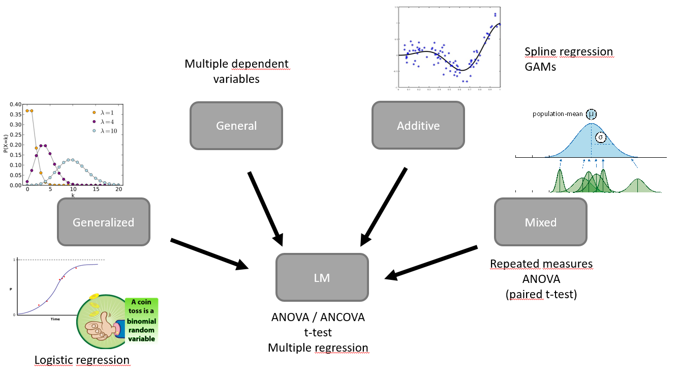
Overview
- Warmup
- Why statistics
- do it yourself statistics
- Linear Regression
- Multiple Regression
- Categorical Variables
- Interactions and the famous 2x2 design
- Inference
- Asumptions
- Bootstrapping
- Four ways of statistics
- Equivalence of traditional tests
Purpose of statistics
- Organization

- Description
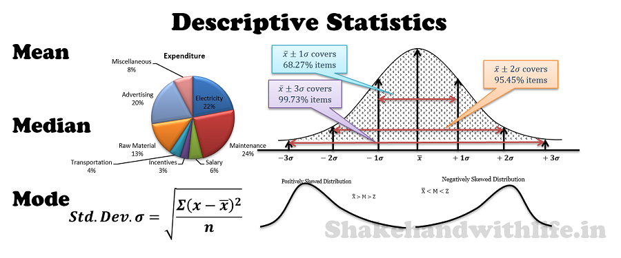
- Inference
Why statistics in the first place?
Because of Variation

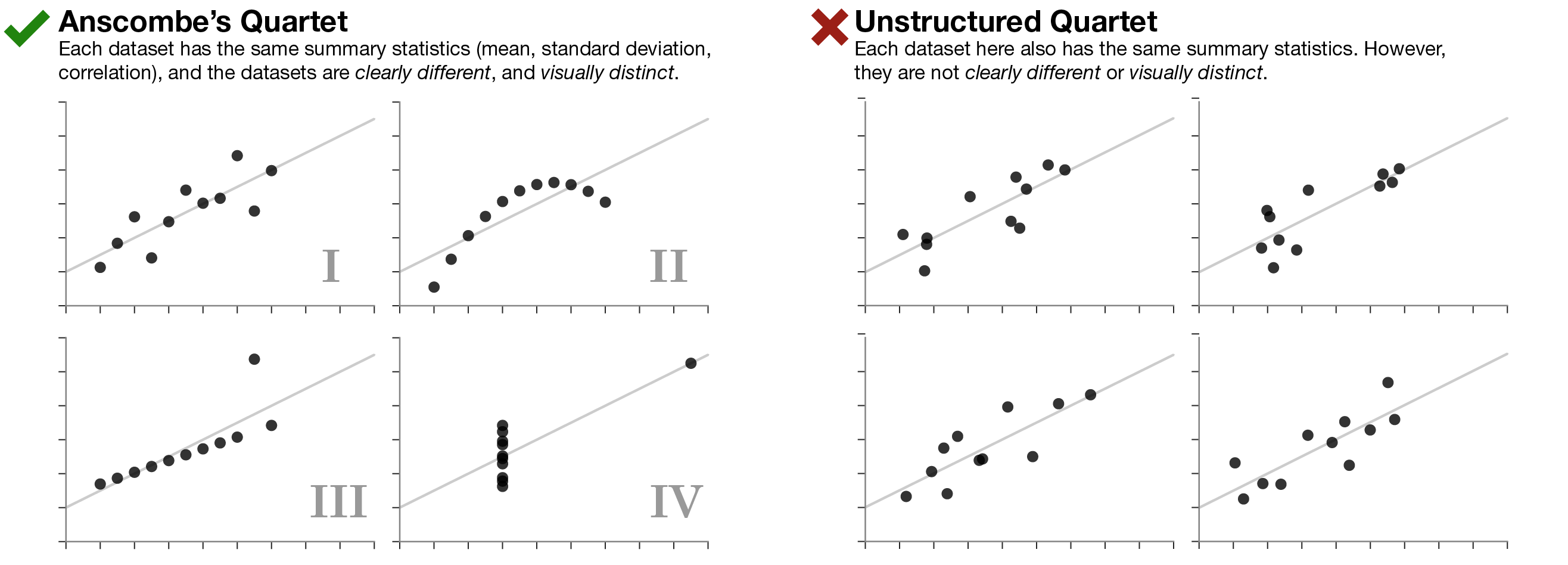
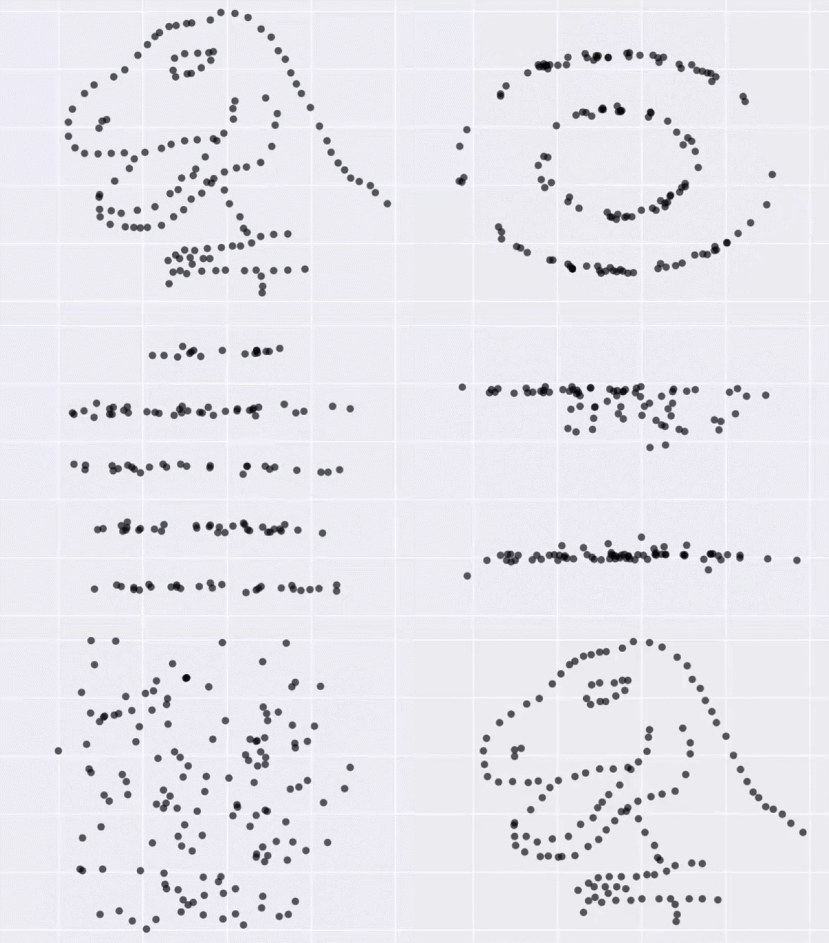
Most important lesson
Always visualize your data
…make both calculations and graphs. Both sorts of output should be studied; each will contribute to understanding. F. J. Anscombe, 1973
Overview
- Warmup
- Why statistics
- do it yourself statistics
- three important concepts
- there is only one statistical test
- Linear Regression
- Multiple Regression
- Categorical Variables
- Interactions and the famous 2x2 design
- Inference
- Asumptions
- Bootstrapping
- Four ways of statistics
- Equivalence of traditional tests
Three extremely important concepts
- Population
- Sample
- Sampling Distribution
Population
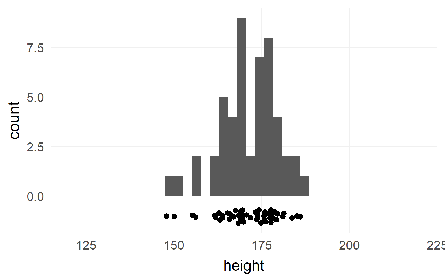
This could be the height of the population
of all people in this room.
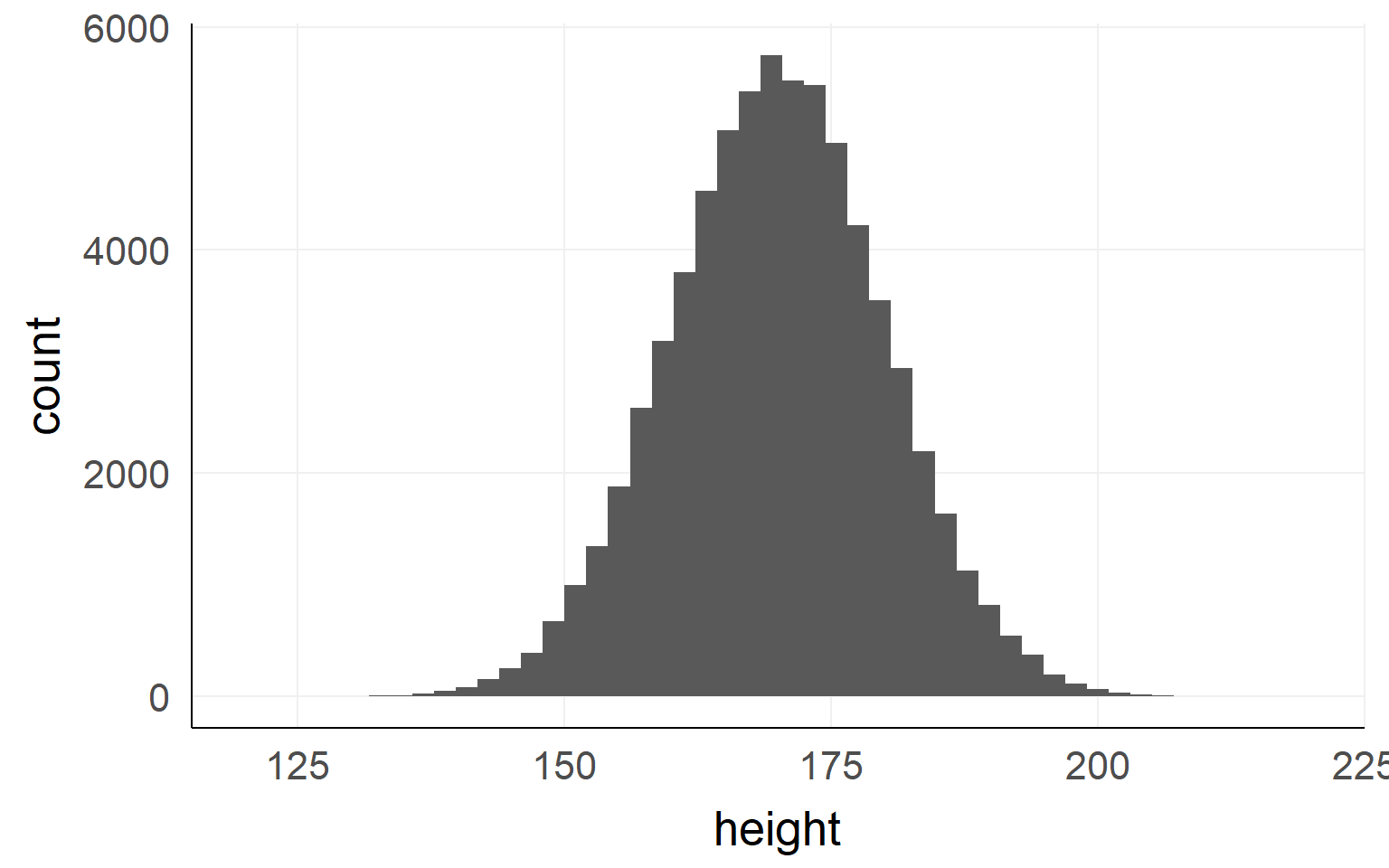
This could be the height of the population of all people in the world. The upper example is a sub-population.
Sample
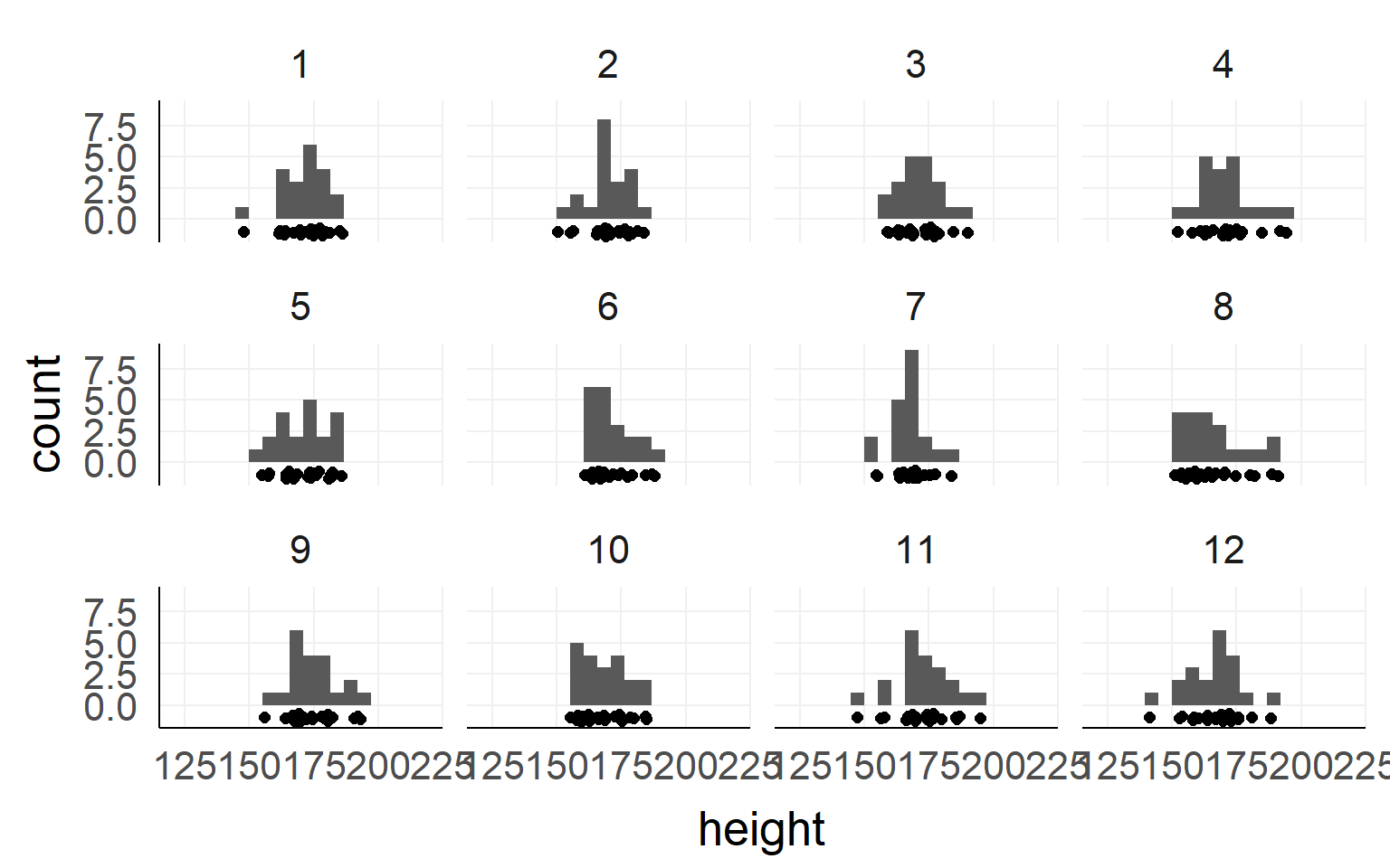
Height measured of 12 different samples (=experiment) of a population.
Sampling Distribution
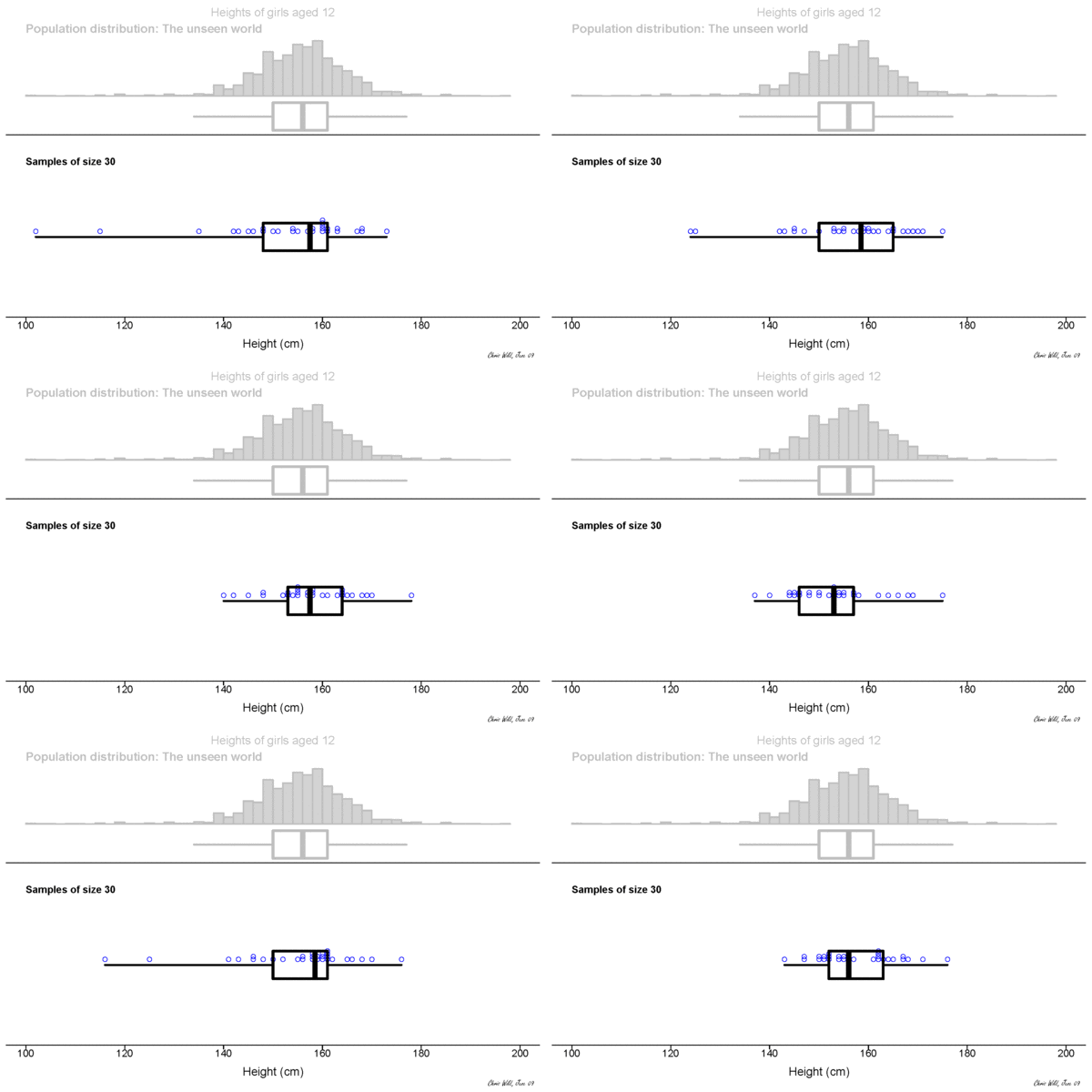
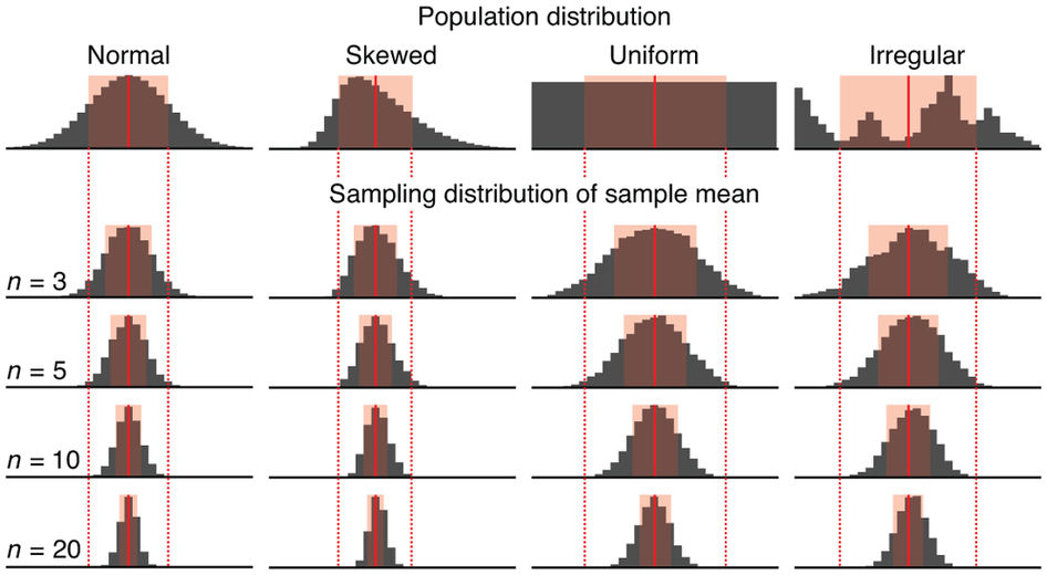
Central limit theorem
Overview
- Warmup
- Why statistics
- do it yourself statistics
- three important concepts
- there is only one statistical test
- Linear Regression
- Multiple Regression
- Categorical Variables
- Interactions and the famous 2x2 design
- Inference
- Asumptions
- Bootstrapping
- Four ways of statistics
- Equivalence of traditional tests
What are statistical inferences?
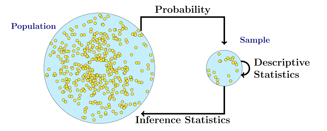
Ingredients for every statistical test
Q:Did our statistic\(^{*}\) occur due to chance\(^{**}\)?
A: To find out, look at the distribution of the statistic at the chance level!
\(^{*}\) could be any measure (statistic), usually: mean, median, variance, t-statistic etc.
\(^{**}\) chance-level is defined by the \(H_0\) (Null Hypothesis), most often it is mean = 0
Example \(n_{obs} = 10\)
##  [1] -0.37645381  0.43364332 -0.58562861  1.84528080  0.57950777
##  [6] -0.57046838  0.73742905  0.98832471  0.82578135 -0.05538839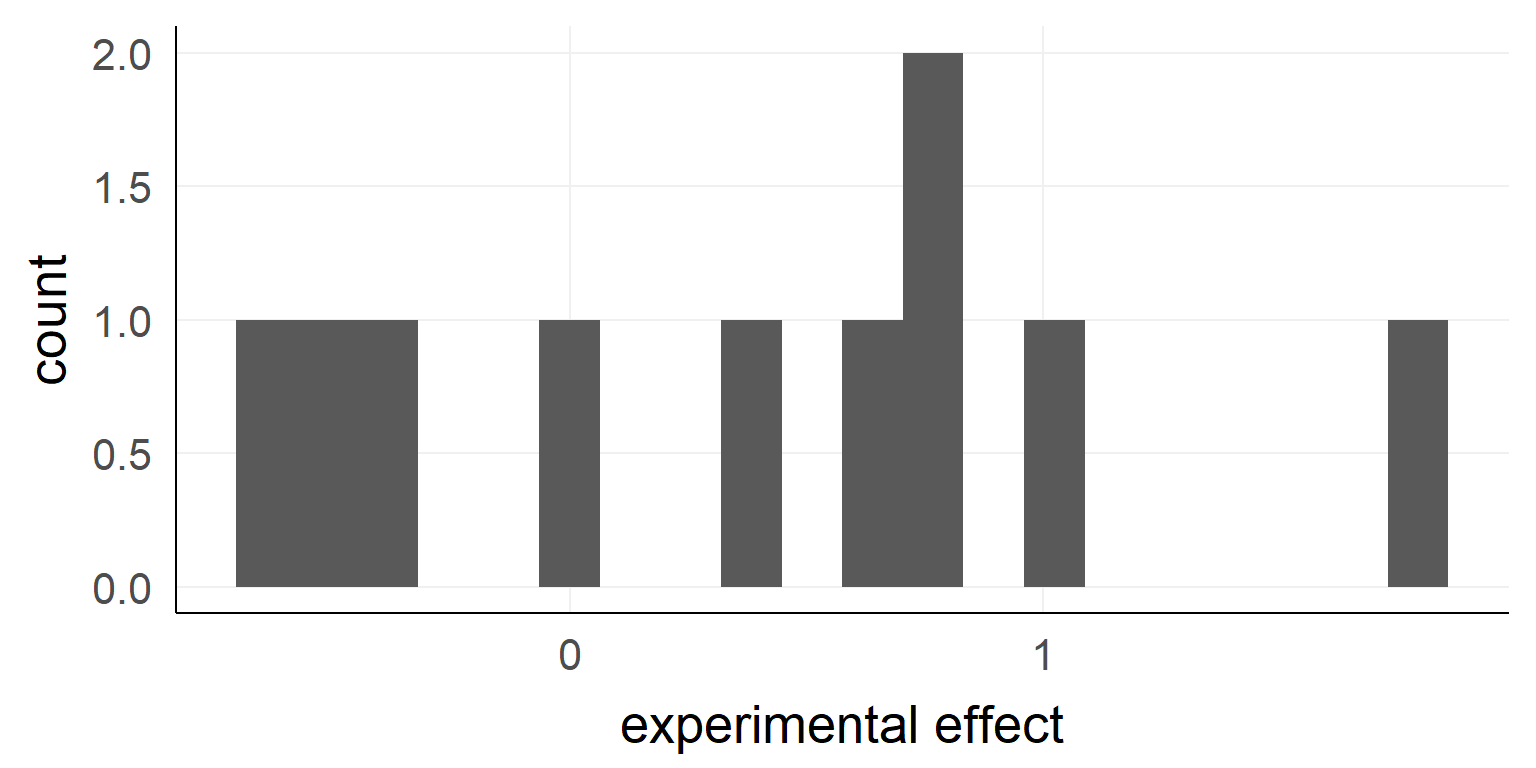
## [1] "mean:0.38, sd:0.78"What we need for our example:
- test-statistic:
- Let’s take the mean value for simplicity (mean(experimental effect) = \(\hat \mu\) = 0.38)
- Chance-Model (commonly called: model of \(H_0\)) - could (in principle) be anything. Let’s assume a normal distribution with a mean of 0 and standard deviation (\(\sigma) = 1\).
The \(H_0\) model
Take 1000 random samples with \(n = n_{obs} = 10\) each
dnull =replicate(1000, rnorm(10) ) %>%reshape2::melt()
null_stat = dnull%>%group_by(Var2)%>%summarise(m = mean(value)) # var2 codes the sample-ID
qplot(null_stat$m,bins=50)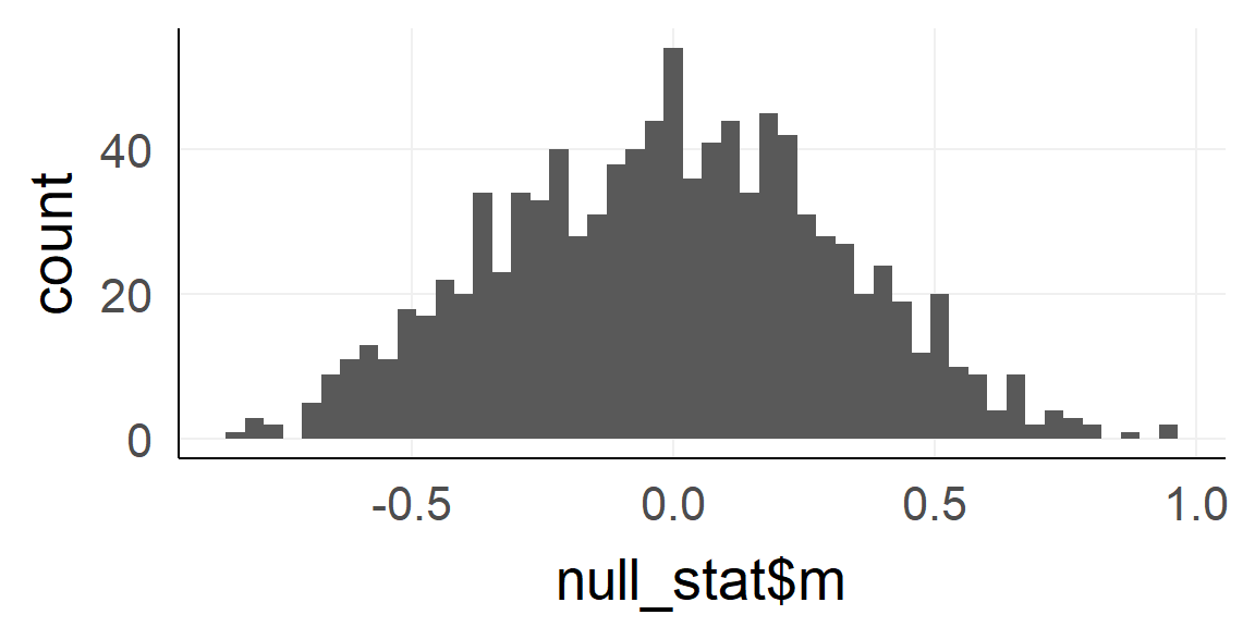
Q: What is this distribution called?
The p-value
Because standardization makes things comparable!
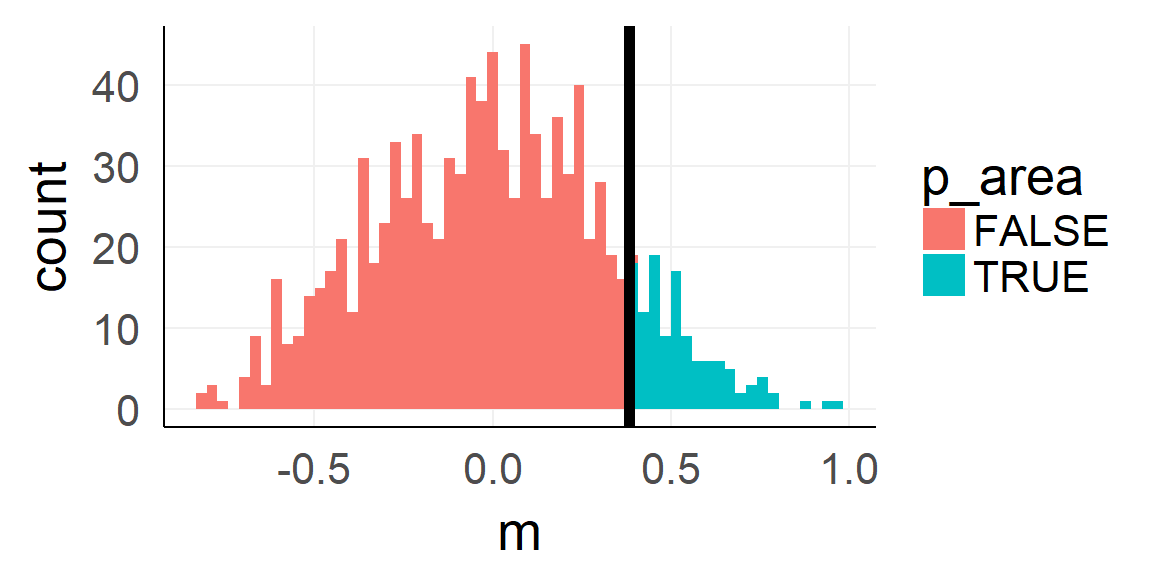
sprintf('p-value: %.3f',sum(null_stat$m >=mean(dobs)) / 1000)## [1] "p-value: 0.121"Analytic shortcut
Simulation can be expensive (e.g. in very complex models => day 4) and computers are needed.

For normal distributed populations (assumption!) the sampling distribution can be easily calculated (a normal with mean = \(mean_{H_0}\), \(SE = \frac{\sigma_{H_0}}{\sqrt N}\), Standard-error)
Summary
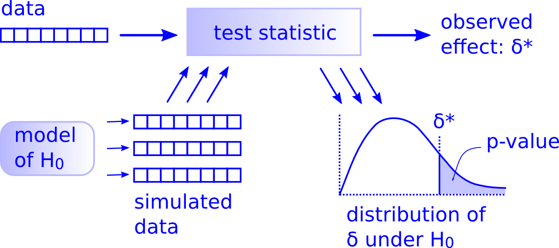
Overview
- Warmup
- Why statistics
- do it yourself statistics
- Introducing the example
- Linear Regression
- Multiple Regression
- Categorical Variables
- Interactions and the famous 2x2 design
- Inference
- Asumptions
- Bootstrapping
- Four ways of statistics
- Equivalence of traditional tests
Should the seatbelt law be withdrawn?

ggplot(data,aes(x=law,y=DriversKilled))+stat_summary()
There could be confounds!
ggplot(data,aes(x=date,y=PetrolPrice,color=factor(law)))+geom_point()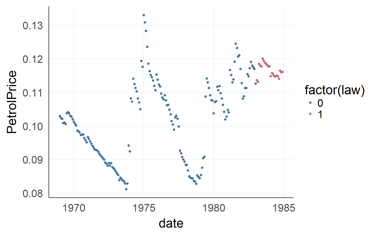 We will ignore the dependency in time. Please never do this in your data - this is an example only! You have been warned
Preview: Multiple regression to the rescue
\(DriversKilled = Average+ kmDrivenEffect + TotalDriverEffect +\) \(PetrolPriceEffect + SeatbeltLawEffect\)
\(DriversKilled = \beta_{average} + \beta_1 \cdot kmsDriven + \beta_2 \cdot TotalDrivers +\) \(\beta_3 \cdot PetrolPrice + \beta_4 \cdot SeatbeltLaw + e_i\)
- Linear Models allow to structure and separate effects
- Linear Models allow to predict values (e.g. what if PetrolPrice would be double the size?)
- Linear Models can be easily extended for non-linear effects (e.g. GAM), complicated distributions(e.g. Yes/No aka logistic regression) or multiple outcomes (General Linear Model)
Overview
- Warmup
- Why statistics
- do it yourself statistics
- Linear Regression
- Multiple Regression
- Categorical Variables
- Interactions and the famous 2x2 design
- Inference
- Asumptions
- Bootstrapping
- Four ways of statistics
- Equivalence of traditional tests
The simple linear regression
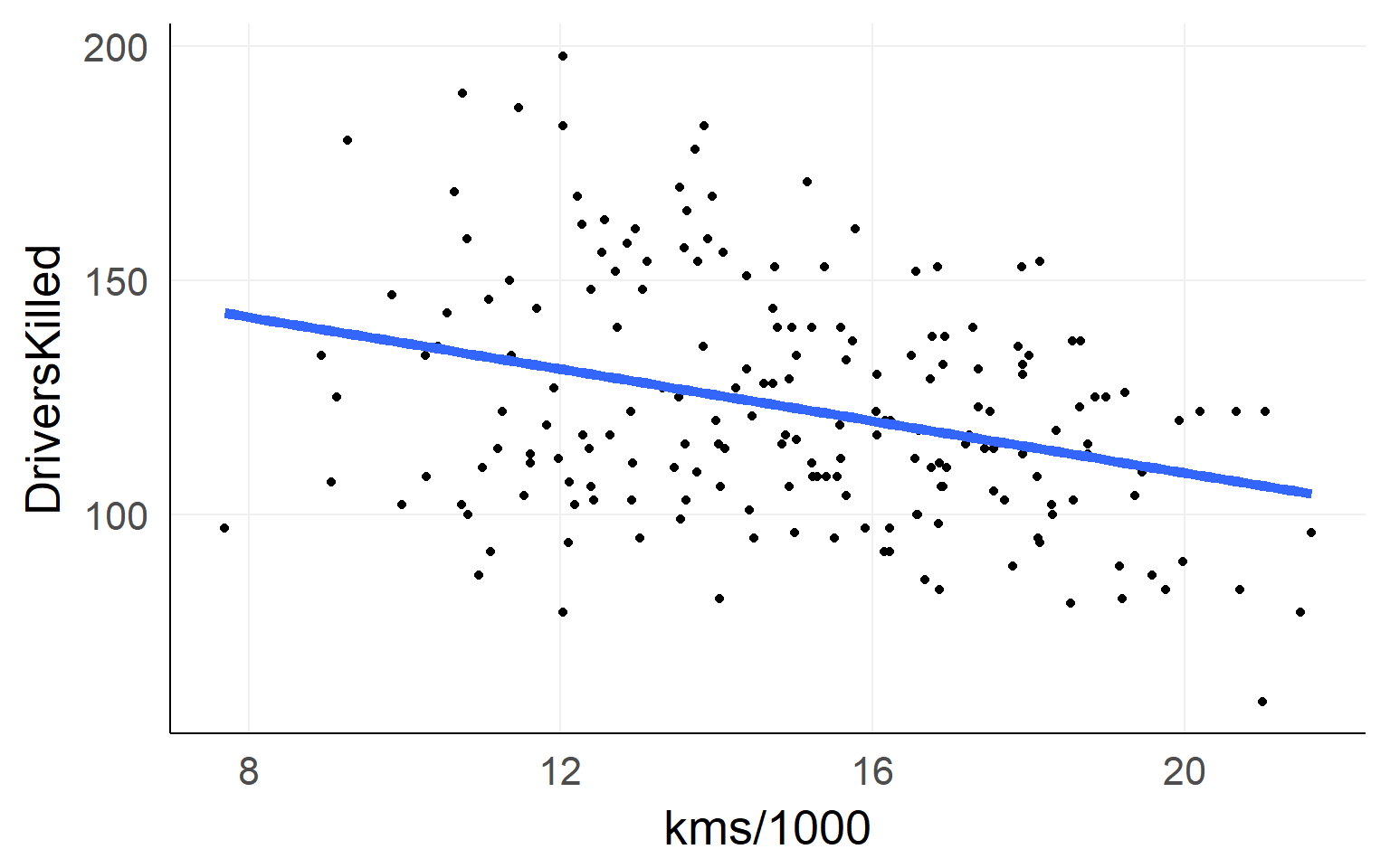
fit = lm(DriversKilled~1+kms,data)Lines are simple! Intercept + Slope
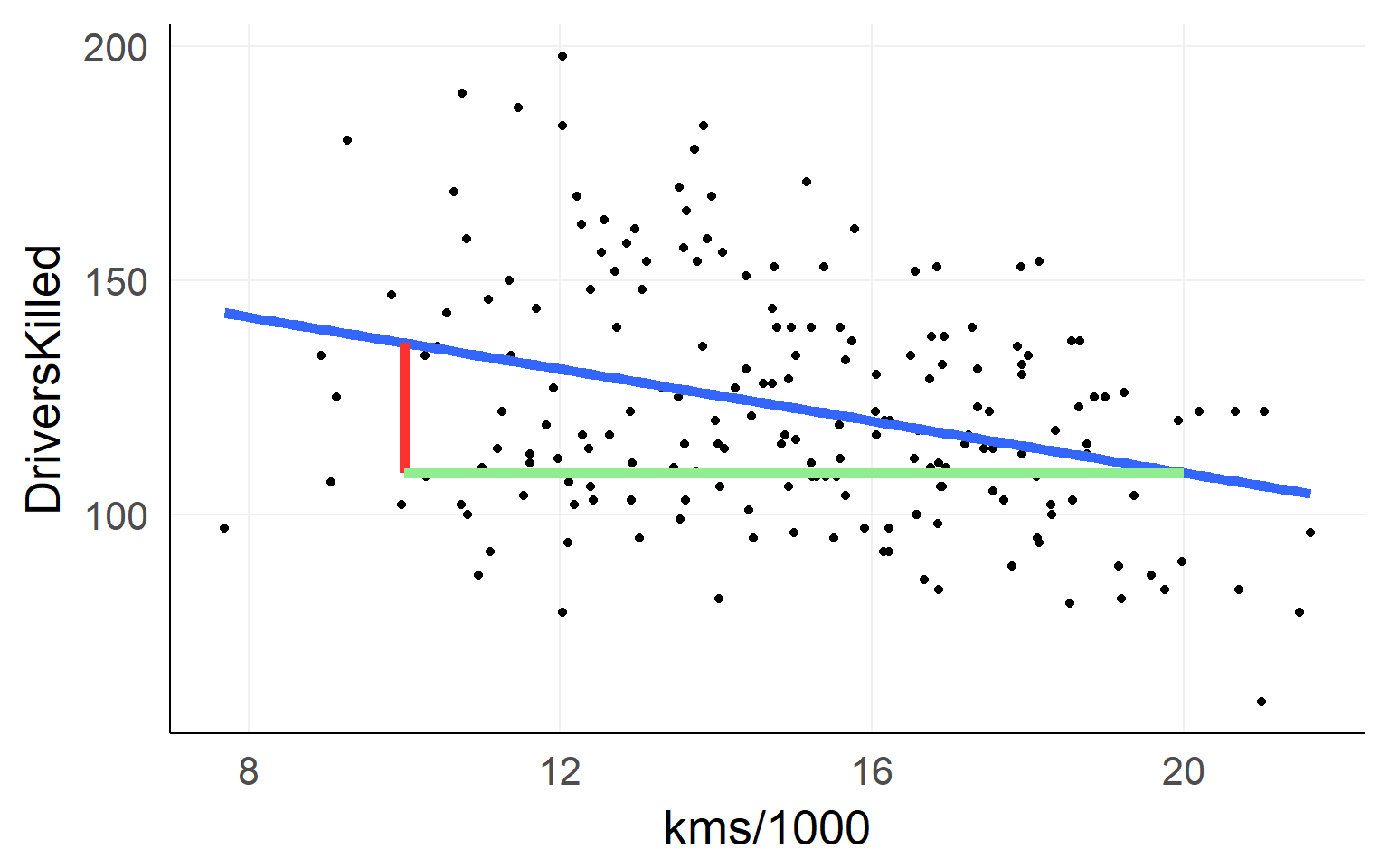
\[ DriversKilled = \beta_0 + (kms/1000) * \beta_1 \]
Red Line: \([DriversKilled | kms/1000==20] - [DriversKilled | kms/1000==10]\)
\(=\beta_0 + 20\beta_1 - (\beta_0 + 10\beta_1)\) \(=10\beta_1\)
Which line to choose?
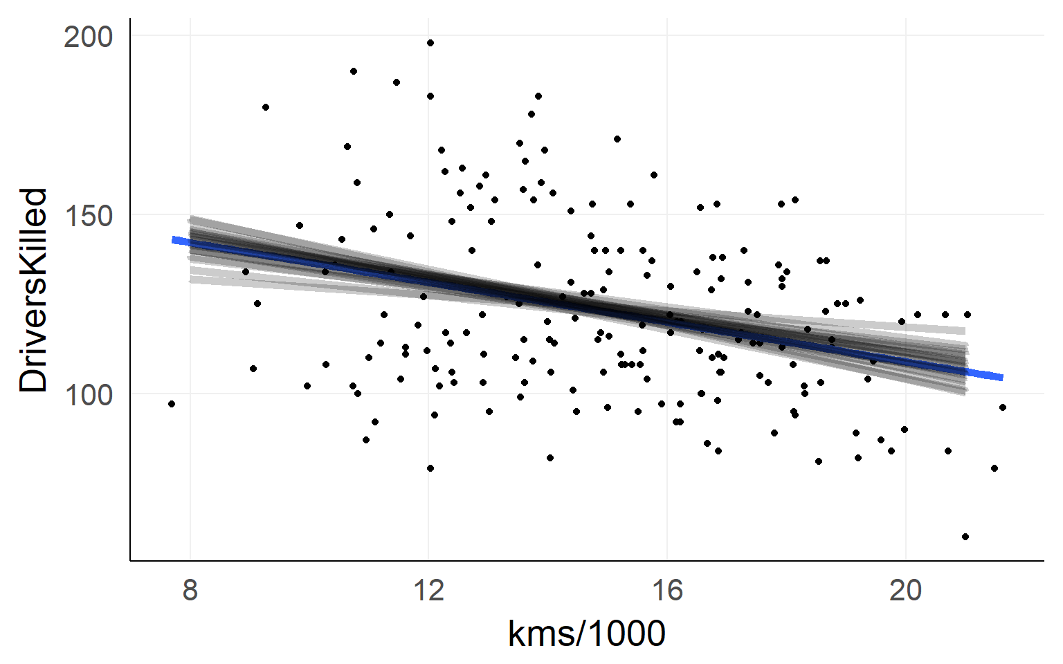
Residuals / L2 Norm
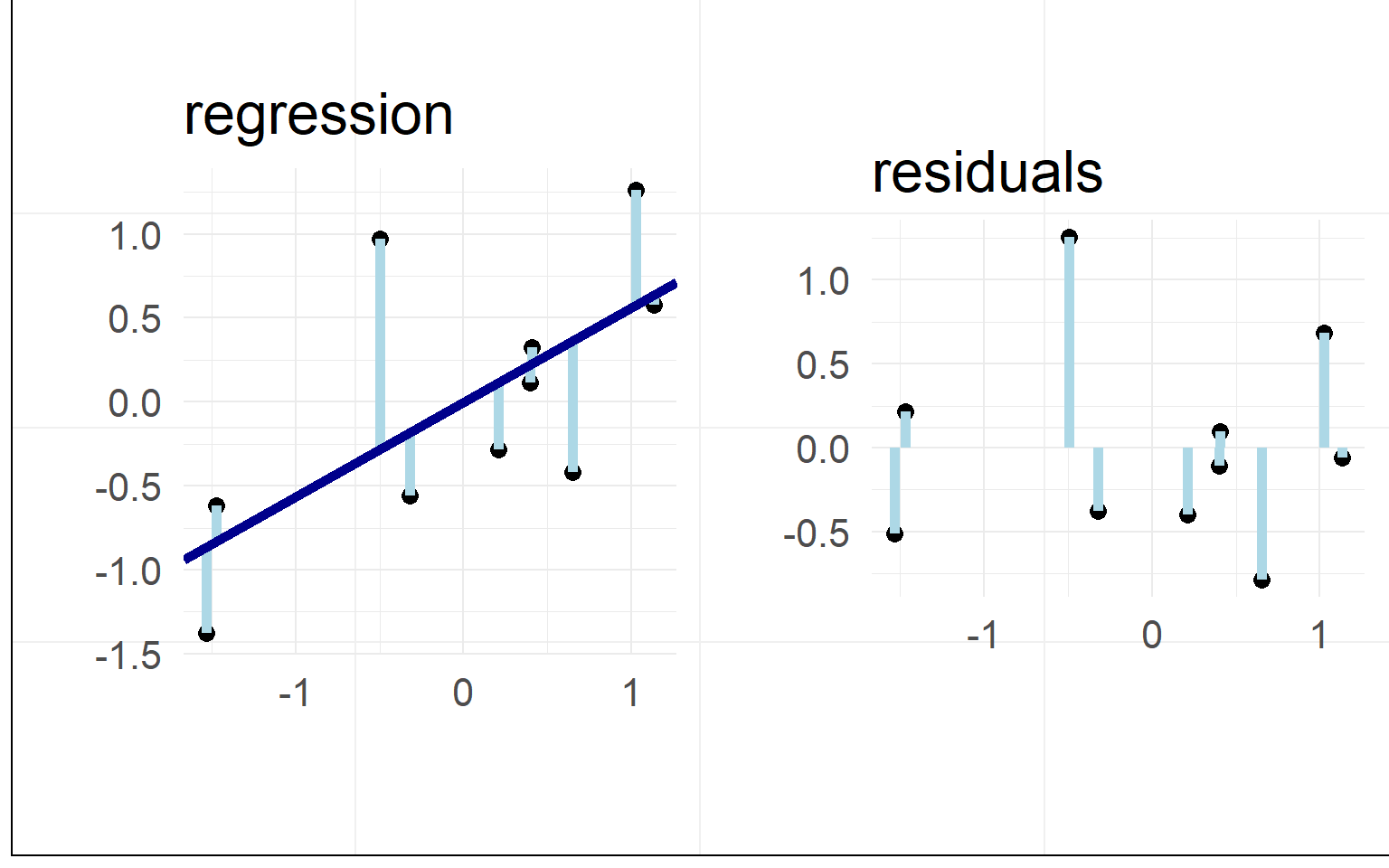
Minimizing the residuals maximizes the fit
L2-Norm (Least Squares): \(min(|residual_i|_2)\)
In our example
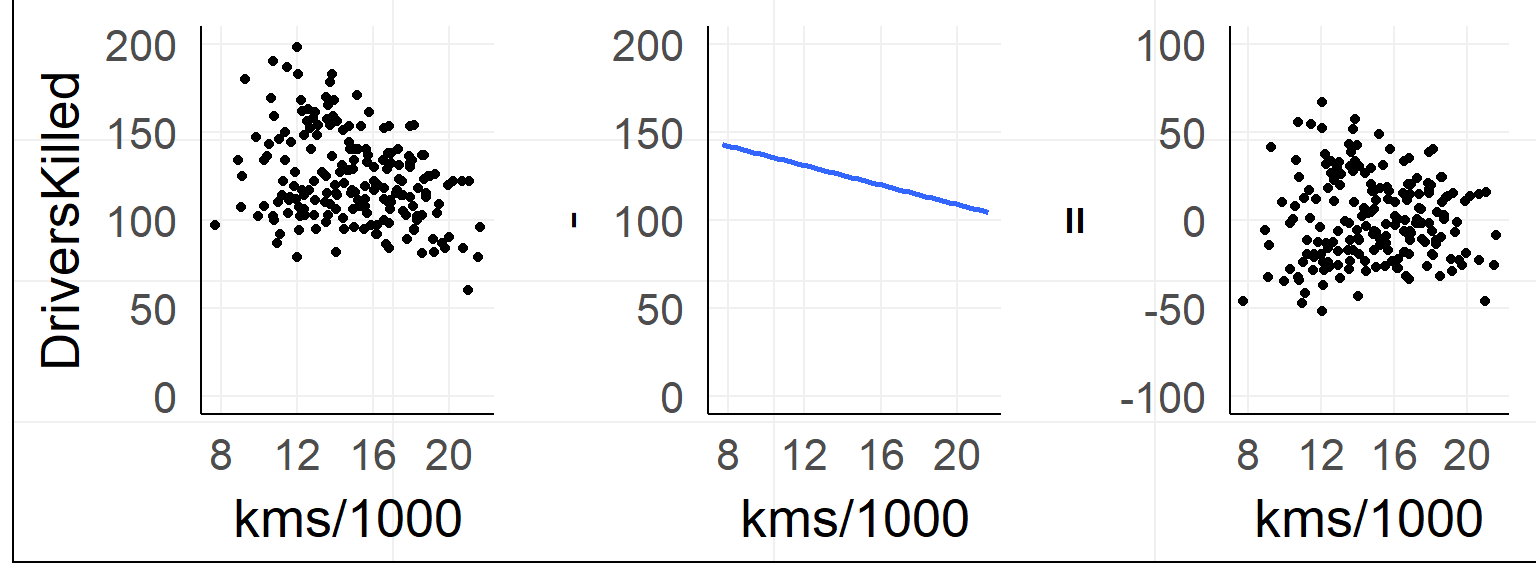
Data: \(y = \beta_0 + x_1 \beta_1 + e_i\)
Prediction: \(\hat{y} = \beta_0 + x_1 \beta_1\)
Residuals: \(e_i = y - \hat{y}\)
in R
summary(lm(formula = DriversKilled ~ 1 + kms,data=data))##
## Call:
## lm(formula = DriversKilled ~ 1 + kms, data = data)
##
## Residuals:
## Min 1Q Median 3Q Max
## -52.028 -19.021 -1.974 16.719 66.964
##
## Coefficients:
## Estimate Std. Error t value Pr(>|t|)
## (Intercept) 1.644e+02 9.067e+00 18.130 < 2e-16 ***
## kms -2.774e-03 5.935e-04 -4.674 5.6e-06 ***
## ---
## Signif. codes: 0 '***' 0.001 '**' 0.01 '*' 0.05 '.' 0.1 ' ' 1
##
## Residual standard error: 24.1 on 190 degrees of freedom
## Multiple R-squared: 0.1031, Adjusted R-squared: 0.09839
## F-statistic: 21.84 on 1 and 190 DF, p-value: 5.596e-06Explained Variance
(I modified the example data for clarity)
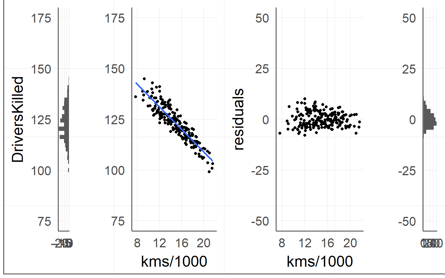
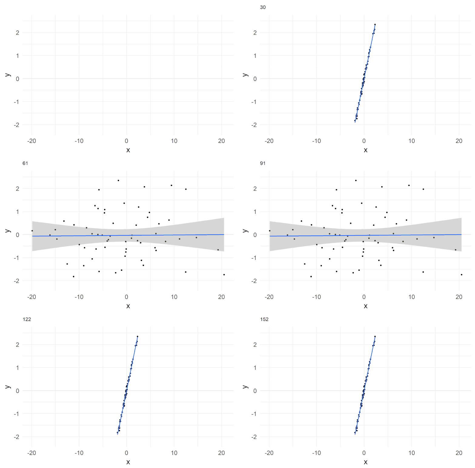
Single outlier
 Especially true for small sample sizes
Overview
- Warmup
- Why statistics
- do it yourself statistics
- Linear Regression
- Multiple Regression
- Categorical Variables
- Interactions and the famous 2x2 design
- Inference
- Asumptions
- Bootstrapping
- Four ways of statistics
- Equivalence of traditional tests

summary(lm(DriversKilled ~ kms + drivers + PetrolPrice,data = data))##
## Call:
## lm(formula = DriversKilled ~ kms + drivers + PetrolPrice, data = data)
##
## Residuals:
## Min 1Q Median 3Q Max
## -27.333 -7.848 -0.532 7.544 35.036
##
## Coefficients:
## Estimate Std. Error t value Pr(>|t|)
## (Intercept) -2.642e+01 1.254e+01 -2.107 0.0365 *
## kms 7.901e-04 3.255e-04 2.428 0.0161 *
## drivers 8.164e-02 3.429e-03 23.810 <2e-16 ***
## PetrolPrice 9.716e+00 7.911e+01 0.123 0.9024
## ---
## Signif. codes: 0 '***' 0.001 '**' 0.01 '*' 0.05 '.' 0.1 ' ' 1
##
## Residual standard error: 11.53 on 188 degrees of freedom
## Multiple R-squared: 0.7969, Adjusted R-squared: 0.7937
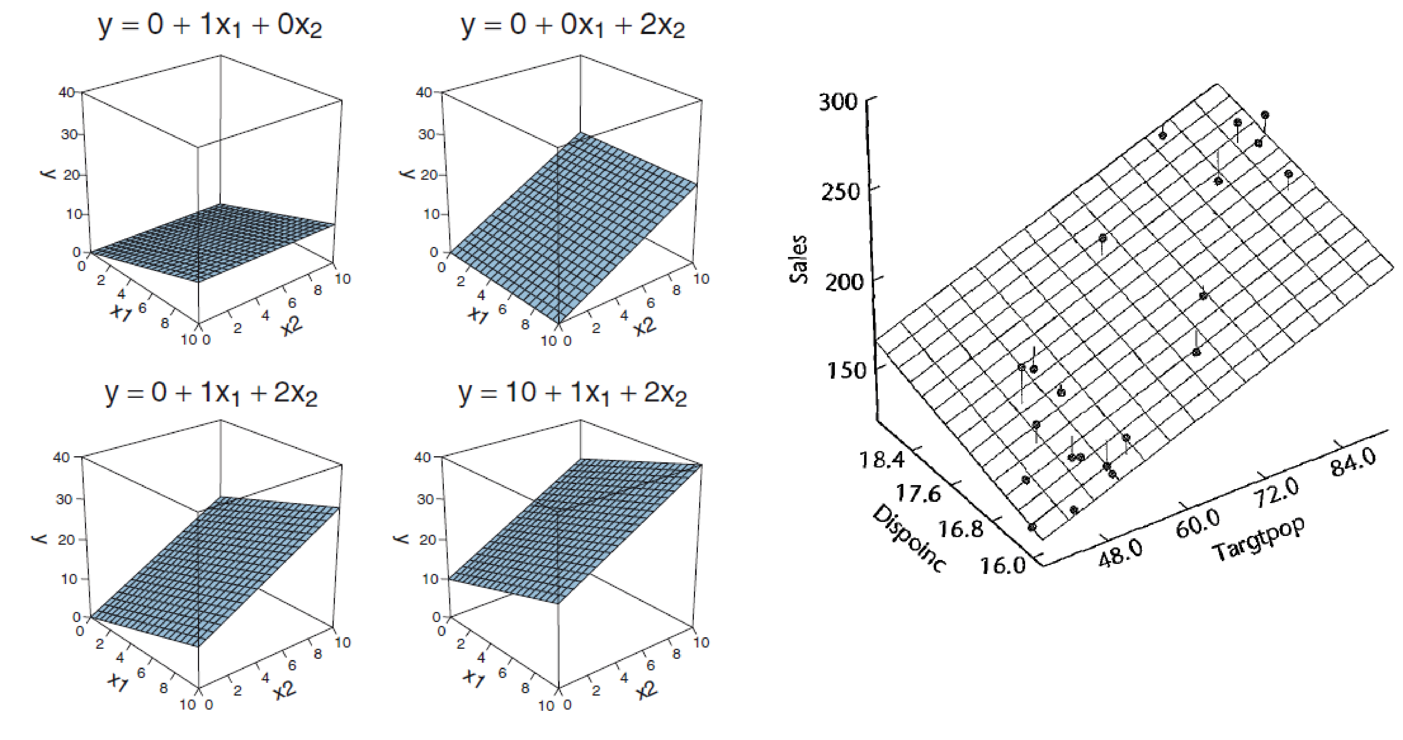
## F-statistic: 245.9 on 3 and 188 DF, p-value: < 2.2e-16With two predictors you span a plane
Overlapping variance
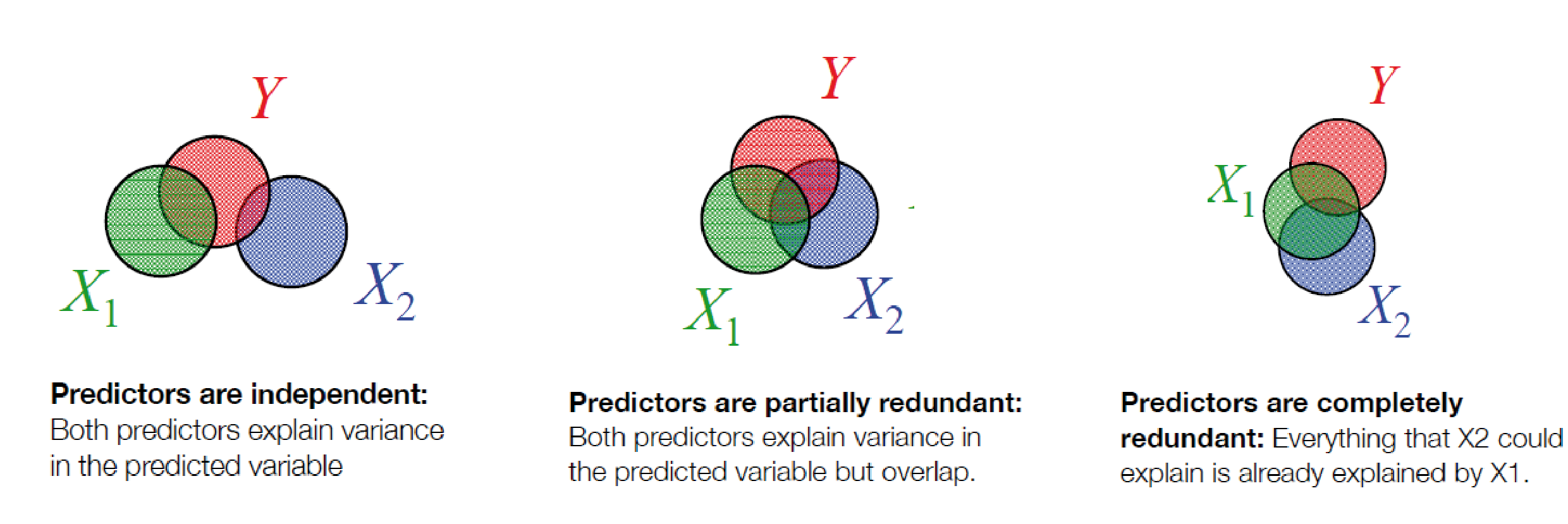
Perfect redundant
data_redundant = data
data_redundant$meters = data_redundant$kms*1000
summary(lm(DriversKilled ~ meters + kms,data = data_redundant))
##
## Call:
## lm(formula = DriversKilled ~ meters + kms, data = data_redundant)
##
## Residuals:
## Min 1Q Median 3Q Max
## -52.028 -19.021 -1.974 16.719 66.964
##
## Coefficients: (1 not defined because of singularities)
## Estimate Std. Error t value Pr(>|t|)
## (Intercept) 1.644e+02 9.067e+00 18.130 < 2e-16 ***
## meters -2.774e-06 5.935e-07 -4.674 5.6e-06 ***
## kms NA NA NA NA
## ---
## Signif. codes: 0 '***' 0.001 '**' 0.01 '*' 0.05 '.' 0.1 ' ' 1
##
## Residual standard error: 24.1 on 190 degrees of freedom
## Multiple R-squared: 0.1031, Adjusted R-squared: 0.09839
## F-statistic: 21.84 on 1 and 190 DF, p-value: 5.596e-06Partially redundant
data_redundant = data
data_redundant$driversnoise = data_redundant$drivers+rnorm(nrow(data_redundant),sd=10)
coef(summary(lm(DriversKilled ~ drivers,data = data_redundant)))
## Estimate Std. Error t value Pr(>|t|)
## (Intercept) -7.30112028 4.938443950 -1.478425 1.409499e-01
## drivers 0.07789178 0.002913364 26.736024 2.636268e-66coef(summary(lm(DriversKilled ~ drivers+driversnoise,data = data_redundant)))## Estimate Std. Error t value Pr(>|t|)
## (Intercept) -7.31191485 4.95029664 -1.4770660 0.1413223
## drivers 0.04903418 0.09120555 0.5376228 0.5914700
## driversnoise 0.02885613 0.09115416 0.3165641 0.7519237Multicollinearity is usually not so obvious
Surpressors: Including unrelated variables can improve modelfit
##
## Call: lm(formula = Y ~ OV + S)
##             Estimate Std. Error t value Pr(>|t|)
## (Intercept) -0.01890    0.01838  -1.028    0.308
## OV           0.99939    0.01798  55.574   <1e-04 ***
## S            0.99859    0.01807  55.252   <1e-04 ***
##
## Residual standard error: 0.1411 on 57 degrees of freedom
## Multiple R-squared:  0.9819, Adjusted R-squared:  0.9812
## F-statistic:  1544 on 2 and 57 DF,  p-value: < 1e-04
##
## Call: lm(formula = Y ~ OV)
## Estimate Std. Error t value Pr(>|t|)
## (Intercept) -0.04080 0.13452 -0.303 0.763
## OV 0.01284 0.01565 0.820 0.415
##
## Residual standard error: 1.033 on 58 degrees of freedom
## Multiple R-squared: 0.01147, Adjusted R-squared: -0.005571
## F-statistic: 0.6731 on 1 and 58 DF, p-value: 0.4153a graphical intuition
A shorthand notation
\(y_i = 1*\beta_0 + x_{i,1}*\beta_1 + x_{i,2}*\beta_2 + ... + x_{i,n}*\beta_n + e_i\)
is nothing else than matrix multiplication
\(y = X\beta+e\)
\(X = designmatrix\) with size \([n_{datapoints},n_{predictors}]\)
\(e = residuals\)with size \([n_{datapoints}]\)Designmatrix & algebra
##     (Intercept)   kms drivers PetrolPrice
## 1             1  9059    1687  0.10297181
## 2             1  7685    1508  0.10236300
## 3             1  9963    1507  0.10206249
## 4             1 10955    1385  0.10087330
## 5             1 11823    1632  0.10101967
## 6             1 12391    1511  0.10058119
## 7             1 13460    1559  0.10377398
## 8             1 14055    1630  0.10407640
## 9             1 12106    1579  0.10377398
## 10            1 11372    1653  0.10302640
## 11            1  9834    2152  0.10273011
## 12            1  9267    2148  0.10199719
## 13            1  9130    1752  0.10127456
## 14            1  8933    1765  0.10070398
## 15            1 11000    1717  0.10013961
## 16            1 10733    1558  0.09862110
## 17            1 12912    1575  0.09834929
## 18            1 12926    1520  0.09808018
## 19            1 13990    1805  0.09727921
## 20            1 14926    1800  0.09741062
## 21            1 12900    1719  0.09742524
## 22            1 12034    2008  0.09638063
## 23            1 10643    2242  0.09573896
## 24            1 10742    2478  0.09510631
## 25            1 10266    2030  0.09673597
## 26            1 10281    1655  0.09610922
## 27            1 11527    1693  0.09536725
## 28            1 12281    1623  0.09470959
## 29            1 13587    1805  0.09411762
## 30            1 13049    1746  0.09353215
## 31            1 16055    1795  0.09295405
## 32            1 15220    1926  0.09283979
## 33            1 13824    1619  0.09272474
## 34            1 12729    1992  0.09226965
## 35            1 11467    2233  0.09170669
## 36            1 11351    2192  0.09126207
## 37            1 10803    2080  0.09071160
## 38            1 10548    1768  0.09027633
## 39            1 12368    1835  0.08995192
## 40            1 13311    1569  0.08909964
## 41            1 13885    1976  0.08867919
## 42            1 14088    1853  0.08815929
## 43            1 16932    1965  0.08890206
## 44            1 16164    1689  0.08818133
## 45            1 14883    1778  0.08894029
## 46            1 13532    1976  0.08772661
## 47            1 12220    2397  0.08742885
## 48            1 12025    2654  0.08703543
## 49            1 11692    2097  0.08644992
## 50            1 11081    1963  0.08587264
## 51            1 13745    1677  0.08539822
## 52            1 14382    1941  0.08382198
## 53            1 14391    2003  0.08459078
## 54            1 15597    1813  0.08413690
## 55            1 16834    2012  0.08377841
## 56            1 17282    1912  0.08351074
## 57            1 15779    2084  0.08280639
## 58            1 13946    2080  0.08117889
## 59            1 12701    2118  0.08285361
## 60            1 10431    2150  0.09419012
## 61            1 11616    1608  0.09239984
## 62            1 10808    1503  0.10816148
## 63            1 12421    1548  0.10721169
## 64            1 13605    1382  0.11404297
## 65            1 14455    1731  0.11245412
## 66            1 15019    1798  0.11131625
## 67            1 15662    1779  0.11030125
## 68            1 16745    1887  0.10819718
## 69            1 14717    2004  0.10702744
## 70            1 13756    2077  0.10494698
## 71            1 12531    2092  0.11935775
## 72            1 12568    2051  0.11762190
## 73            1 11249    1577  0.13302742
## 74            1 11096    1356  0.13084524
## 75            1 12637    1652  0.12831848
## 76            1 13018    1382  0.12354745
## 77            1 15005    1519  0.11858681
## 78            1 15235    1421  0.11633748
## 79            1 15552    1442  0.11516148
## 80            1 16905    1543  0.11450120
## 81            1 14776    1656  0.11352298
## 82            1 14104    1561  0.11193018
## 83            1 12854    1905  0.11061053
## 84            1 12956    2199  0.11527439
## 85            1 12177    1473  0.11379349
## 86            1 11918    1655  0.11234958
## 87            1 13517    1407  0.11175347
## 88            1 14417    1395  0.10964252
## 89            1 15911    1530  0.10844090
## 90            1 15589    1309  0.10788494
## 91            1 16543    1526  0.10908477
## 92            1 17925    1327  0.10757145
## 93            1 15406    1627  0.10616402
## 94            1 14601    1748  0.10630000
## 95            1 13107    1958  0.10482531
## 96            1 12268    2274  0.10345175
## 97            1 11972    1648  0.10144992
## 98            1 12028    1401  0.10040232
## 99            1 14033    1411  0.09886203
## 100           1 14244    1403  0.10249615
## 101           1 15287    1394  0.10302743
## 102           1 16954    1520  0.10217891
## 103           1 17361    1528  0.09983664
## 104           1 17694    1643  0.09263669
## 105           1 16222    1515  0.09181496
## 106           1 14969    1685  0.09072430
## 107           1 13624    2000  0.09002121
## 108           1 13842    2215  0.08933071
## 109           1 12387    1956  0.08844273
## 110           1 11608    1462  0.08835257
## 111           1 15021    1563  0.08675736
## 112           1 14834    1459  0.08499524
## 113           1 16565    1446  0.08456794
## 114           1 16882    1622  0.08443190
## 115           1 18012    1657  0.08435088
## 116           1 18855    1638  0.08360098
## 117           1 17243    1643  0.08341726
## 118           1 16045    1683  0.08274514
## 119           1 14745    2050  0.08523527
## 120           1 13726    2262  0.08477030
## 121           1 11196    1813  0.08445892
## 122           1 12105    1445  0.08535212
## 123           1 14723    1762  0.08755921
## 124           1 15582    1461  0.09038292
## 125           1 16863    1556  0.09078329
## 126           1 16758    1431  0.10874278
## 127           1 17434    1427  0.11414223
## 128           1 18359    1554  0.11299293
## 129           1 17189    1645  0.11132071
## 130           1 16909    1653  0.10912623
## 131           1 15380    2016  0.10769846
## 132           1 15161    2207  0.10760157
## 133           1 14027    1665  0.10377502
## 134           1 14478    1361  0.10711417
## 135           1 16155    1506  0.10737477
## 136           1 16585    1360  0.11169537
## 137           1 18117    1453  0.11063818
## 138           1 17552    1522  0.11185521
## 139           1 18299    1460  0.10974234
## 140           1 19361    1552  0.10819393
## 141           1 17924    1548  0.10625536
## 142           1 17872    1827  0.10419303
## 143           1 16058    1737  0.10193397
## 144           1 15746    1941  0.10279382
## 145           1 15226    1474  0.10476034
## 146           1 14932    1458  0.10400254
## 147           1 16846    1542  0.11665552
## 148           1 16854    1404  0.11516148
## 149           1 18146    1522  0.11298954
## 150           1 17559    1385  0.11386064
## 151           1 18655    1641  0.11911808
## 152           1 19453    1510  0.12448999
## 153           1 17923    1681  0.12322295
## 154           1 17915    1938  0.12067793
## 155           1 16496    1868  0.12104898
## 156           1 13544    1726  0.11696857
## 157           1 13601    1456  0.11275026
## 158           1 15667    1445  0.10807931
## 159           1 17358    1456  0.10883852
## 160           1 18112    1365  0.11129177
## 161           1 18581    1487  0.11130401
## 162           1 18759    1558  0.11545436
## 163           1 20668    1488  0.11476830
## 164           1 21040    1684  0.11720743
## 165           1 18993    1594  0.11907640
## 166           1 18668    1850  0.11796586
## 167           1 16768    1998  0.11744913
## 168           1 16551    2079  0.11698846
## 169           1 16231    1494  0.11261054
## 170           1 15511    1057  0.11365702
## 171           1 18308    1218  0.11314445
## 172           1 17793    1168  0.11849553
## 173           1 19205    1236  0.11796940
## 174           1 19162    1076  0.11768661
## 175           1 20997    1174  0.12005924
## 176           1 20705    1139  0.11943775
## 177           1 18759    1427  0.11888127
## 178           1 19240    1487  0.11846236
## 179           1 17504    1483  0.11801660
## 180           1 16591    1513  0.11770662
## 181           1 16224    1357  0.11777609
## 182           1 16670    1165  0.11479699
## 183           1 18539    1282  0.11573525
## 184           1 19759    1110  0.11535626
## 185           1 19584    1297  0.11481536
## 186           1 19976    1185  0.11477748
## 187           1 21486    1222  0.11493598
## 188           1 21626    1284  0.11479699
## 189           1 20195    1444  0.11409316
## 190           1 19928    1575  0.11646552
## 191           1 18564    1737  0.11602611
## 192           1 18149    1763  0.11606673
\[ y = X\beta\] Can be solved by: \[ \beta = (X^TX)^{-1}X^Ty\] (don’t memorize this)
Overview
- Warmup
- Why statistics
- do it yourself statistics
- Linear Regression
- Multiple Regression
- Categorical Variables
- Interactions and the famous 2x2 design
- Inference
- Asumptions
- Bootstrapping
- Four ways of statistics
- Equivalence of traditional tests
Dummy Coding
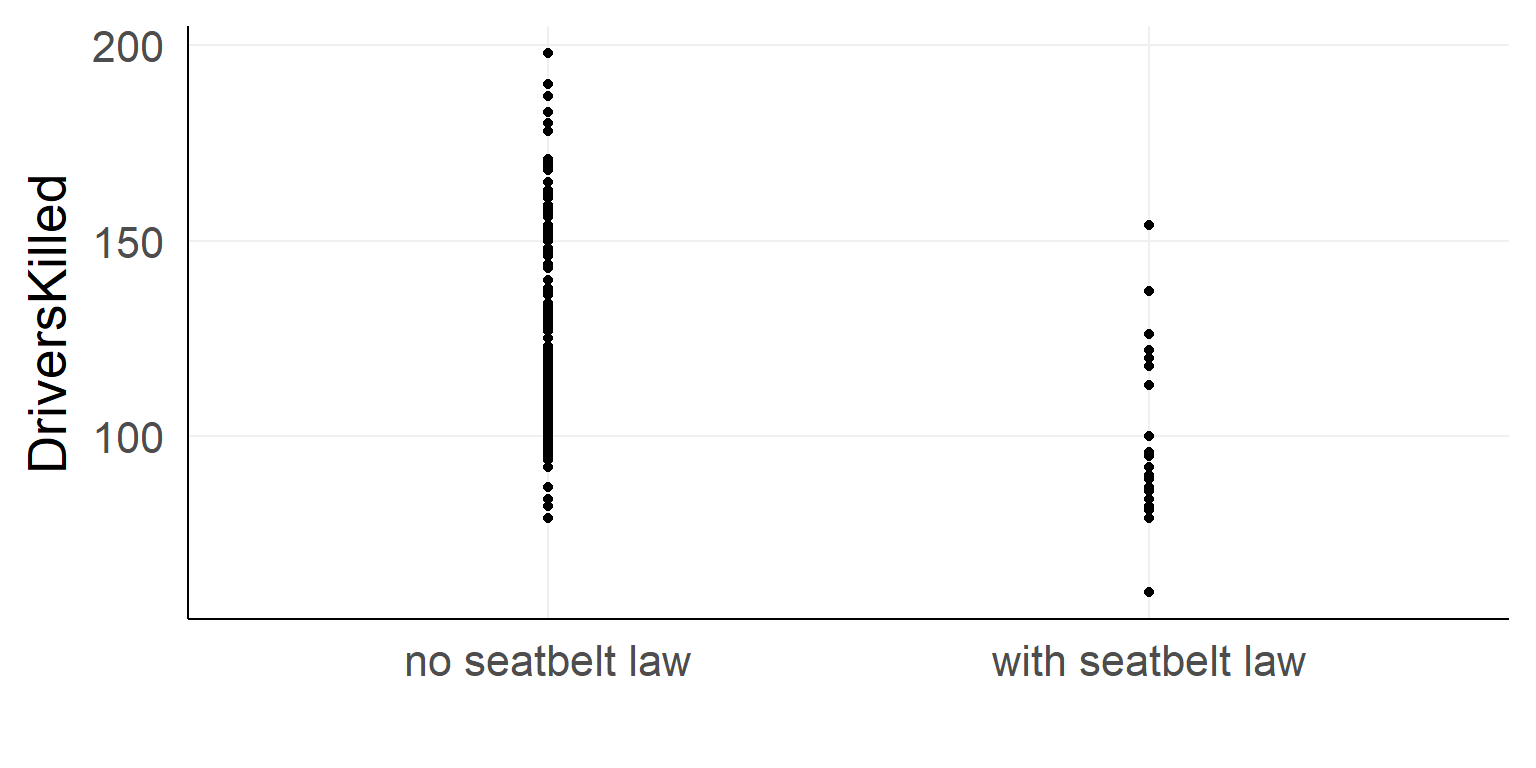
Dummy Coding
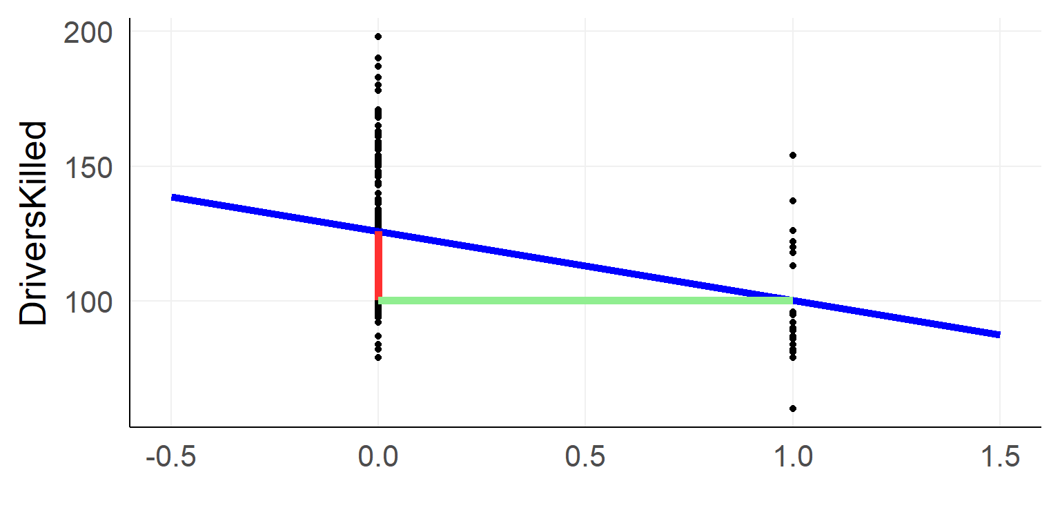
We code the categorical variable with 0 / 1
\(y_i = \beta_0 + is\_law *\beta_1 + e_i\)
Interpretation
\(y_i = \beta_0 + is\_law *\beta_1 + e_i\)
- \(\beta_0\) / Intercept: Driverskilled when \(is\_law\) equals 0
- \(\beta_1\) / Slope: Additional drivers killed when \(is\_law\) was changed to 1
summary(lm(data=data_factor,DriversKilled~1+law))##
## Call:
## lm(formula = DriversKilled ~ 1 + law, data = data_factor)
##
## Residuals:
## Min 1Q Median 3Q Max
## -46.870 -17.870 -5.565 14.130 72.130
##
## Coefficients:
## Estimate Std. Error t value Pr(>|t|)
## (Intercept) 125.870 1.849 68.082 < 2e-16 ***
## lawwith seatbelt law -25.609 5.342 -4.794 3.29e-06 ***
## ---
## Signif. codes: 0 '***' 0.001 '**' 0.01 '*' 0.05 '.' 0.1 ' ' 1
##
## Residual standard error: 24.03 on 190 degrees of freedom
## Multiple R-squared: 0.1079, Adjusted R-squared: 0.1032
## F-statistic: 22.98 on 1 and 190 DF, p-value: 3.288e-06Effect Coding aka sum coding aka deviation coding
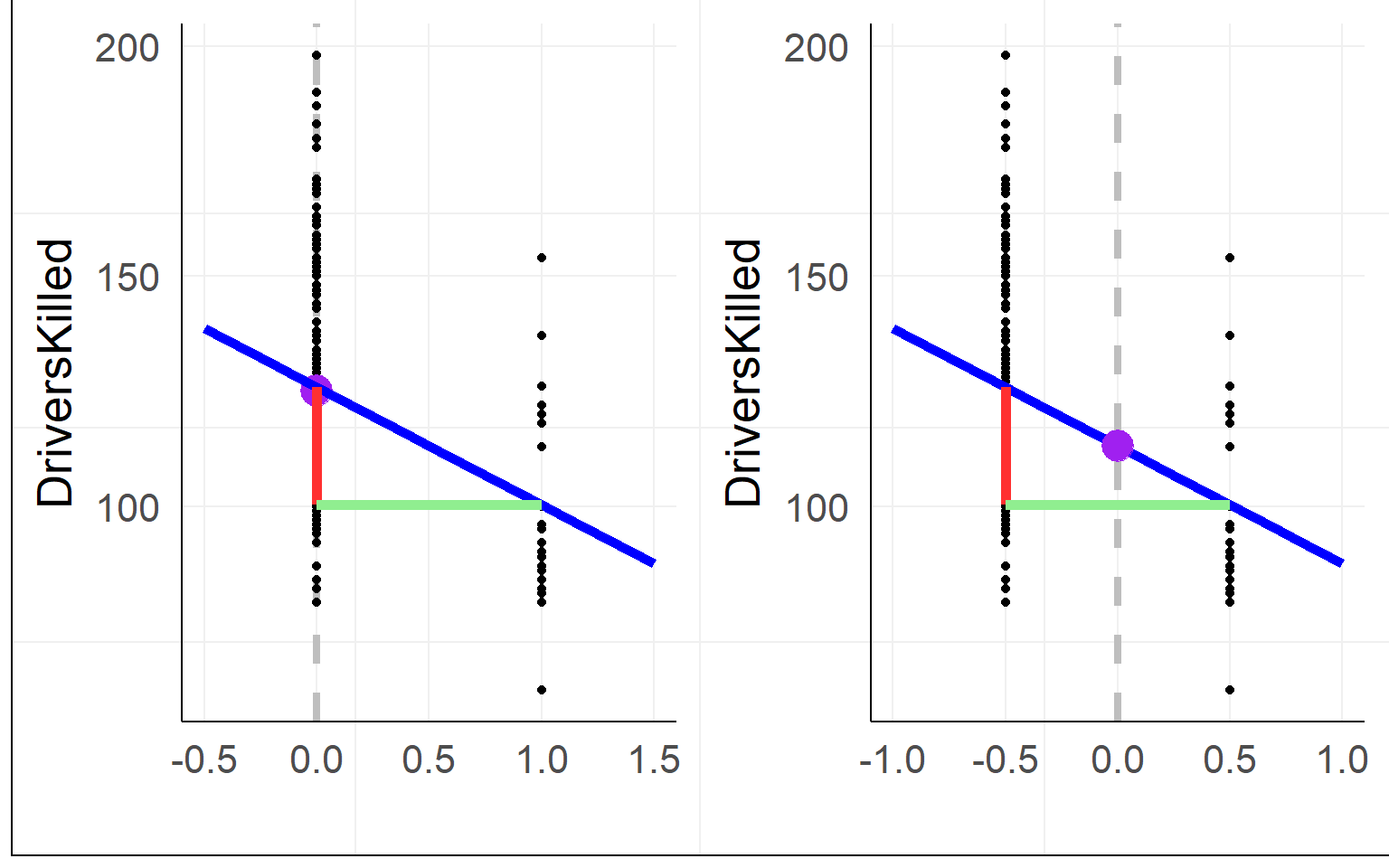
Using effect coding, the interpretation of the intercept changes to the mean between groups
warning: often effect coding is made using -1 and 1, then the \(\beta_1\) is halve the size! using 0.5 is much more practicalMultiple levels
| (Intercept) | factormiddle | factorhigh |
|---|---|---|
| 1 | 0 | 0 |
| 1 | 0 | 0 |
| 1 | 0 | 0 |
| 1 | 1 | 0 |
| 1 | 1 | 0 |
| 1 | 1 | 0 |
| 1 | 0 | 1 |
| 1 | 0 | 1 |
| 1 | 0 | 1 |
Treatment / Dummy Coding
| (Intercept) | factor1 | factor2 |
|---|---|---|
| 1 | 0.5 | 0.0 |
| 1 | 0.5 | 0.0 |
| 1 | 0.5 | 0.0 |
| 1 | 0.0 | 0.5 |
| 1 | 0.0 | 0.5 |
| 1 | 0.0 | 0.5 |
| 1 | -0.5 | -0.5 |
| 1 | -0.5 | -0.5 |
| 1 | -0.5 | -0.5 |
Effect Coding
Overview
- Warmup
- Why statistics
- do it yourself statistics
- Linear Regression
- Multiple Regression
- Categorical Variables
- Interactions and the famous 2x2 design
- Inference
- Asumptions
- Bootstrapping
- Four ways of statistics
- Equivalence of traditional tests
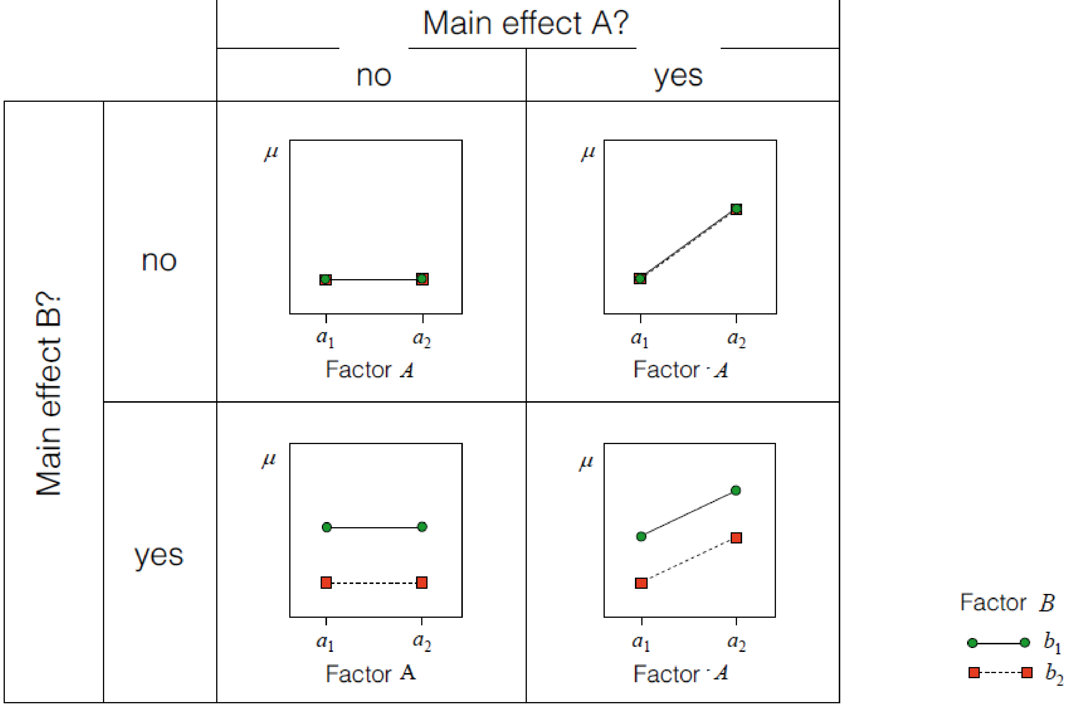 errorbars/data-points ommited for clarity
Interaction effects
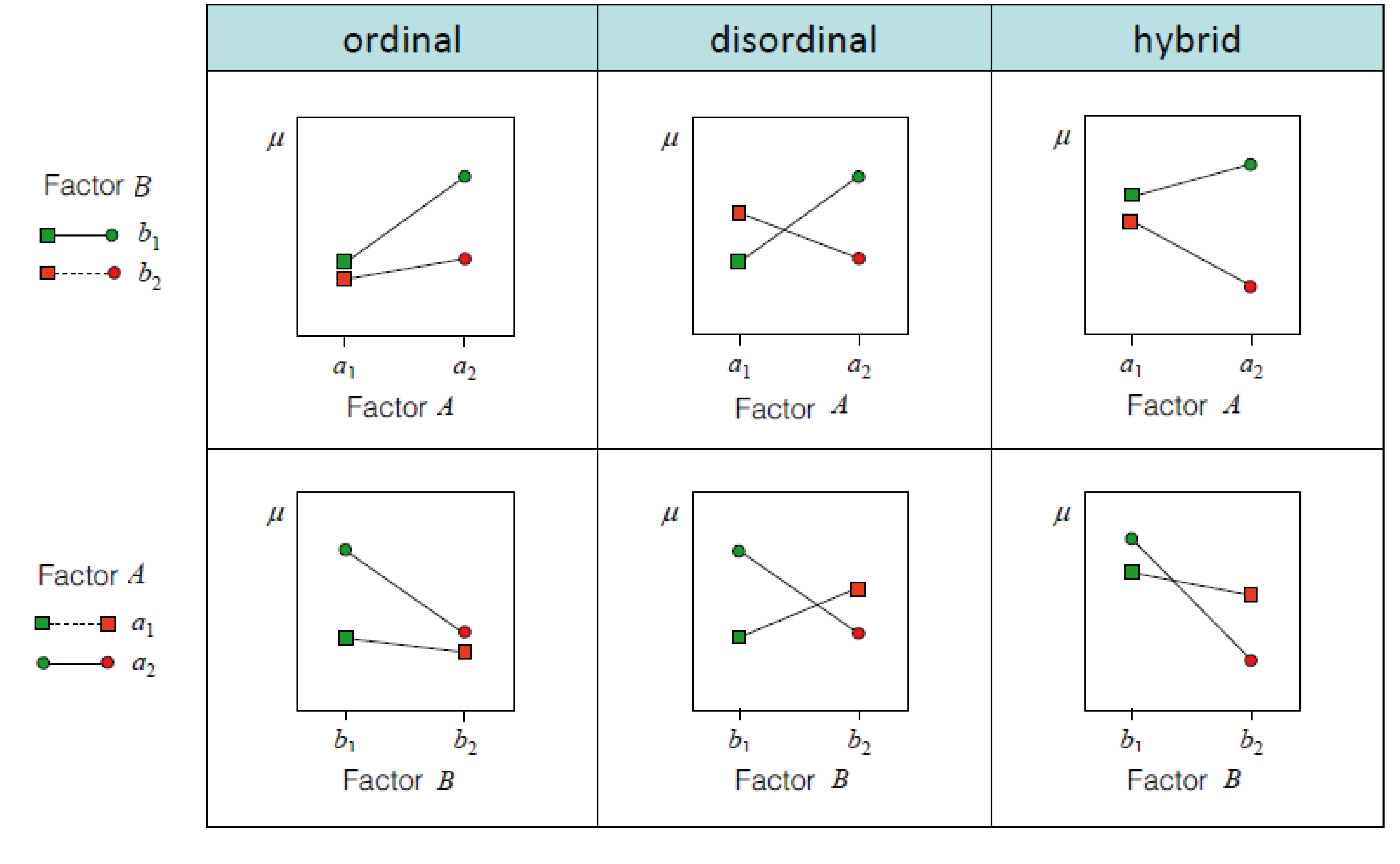
How are interactions coded
\(y = \beta_0 + factorA * \beta_1 + factorB * \beta_2 + factorA * factorB * \beta_3\)
Different words for the same thing:
- The interaction shows how much the prediction needs to be changed, when both factors coocur
- The interaction is the multiplication of the columns in X of factorA and factorB
- The interaction represents the difference of differences
Interactions of continuous/categorical predicotrs
\(y = \beta_0 + factorA * \beta_1 + contB * \beta_2 + factorA * contB * \beta_3\) 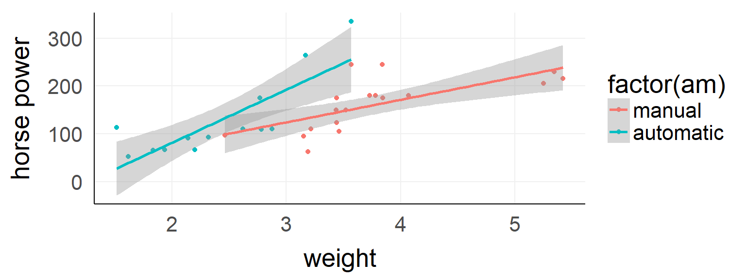
##
## Call: lm(formula = hp ~ wt * am, data = d)
##             Estimate Std. Error t value Pr(>|t|)
## (Intercept)   -17.39      52.44  -0.332  0.74260
## wt             47.14      13.64   3.456  0.00177 **
## am           -123.33      74.03  -1.666  0.10690
## wt:am          63.84      25.08   2.545  0.01672 *
##
## Residual standard error: 44.99 on 28 degrees of freedom
## Multiple R-squared:  0.6111, Adjusted R-squared:  0.5694
## F-statistic: 14.66 on 3 and 28 DF, p-value: < 1e-04The difference between main and simple effects
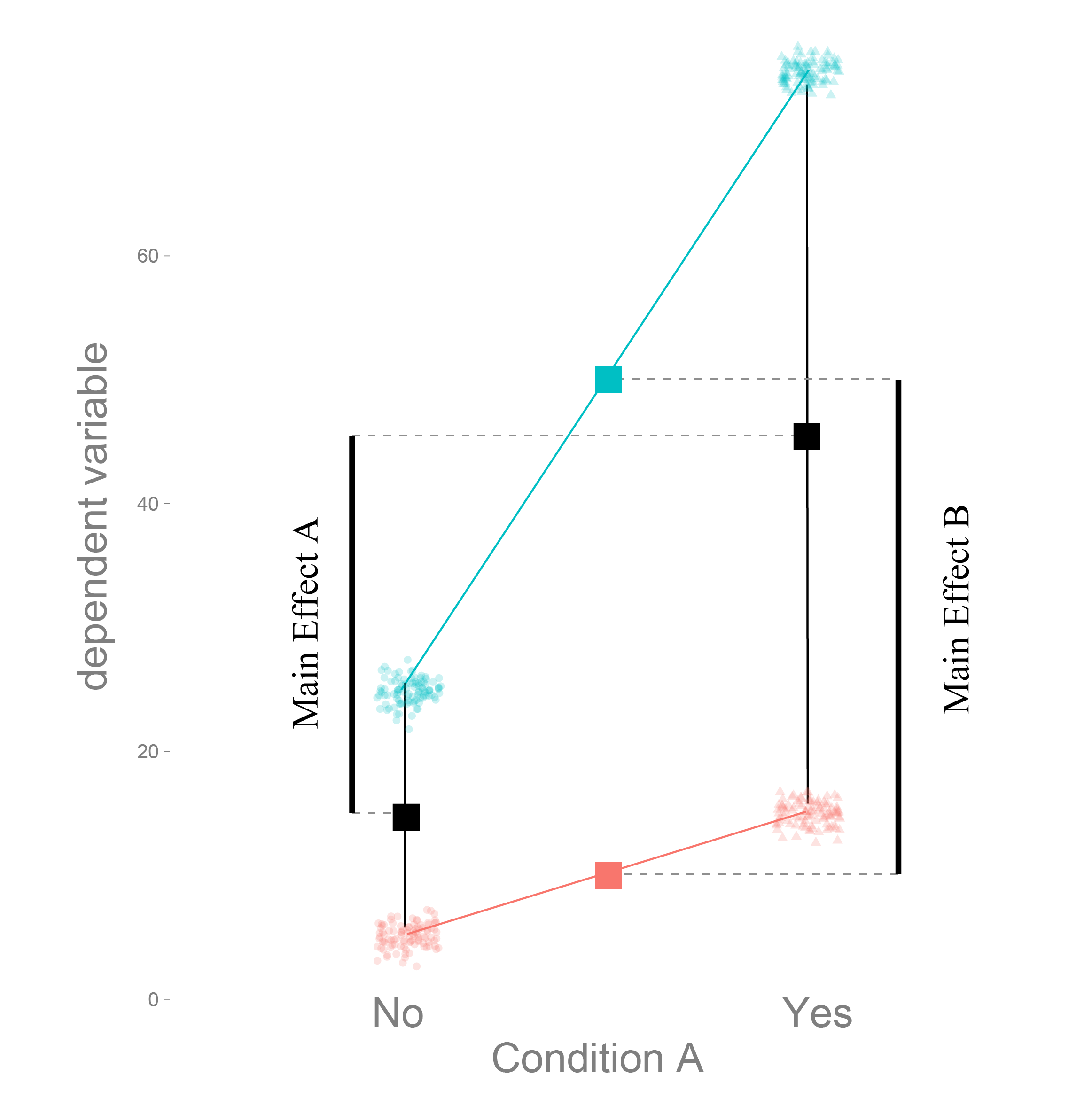
Dummy coding tests simple effects
Effect coding main effects
Effect coding to the help!
##
## Call: lm(formula = hp ~ wt * am, data = d)
##             Estimate Std. Error t value Pr(>|t|)
## (Intercept)   -17.39      52.44  -0.332  0.74260
## wt             47.14      13.64   3.456  0.00177 **
## am           -123.33      74.03  -1.666  0.10690
## wt:am          63.84      25.08   2.545  0.01672 *
##
## Residual standard error: 44.99 on 28 degrees of freedom
## Multiple R-squared:  0.6111, Adjusted R-squared:  0.5694
## F-statistic: 14.66 on 3 and 28 DF,  p-value: < 1e-04
##
## Call: lm(formula = hp ~ wt * am, data = d)
## Estimate Std. Error t value Pr(>|t|)
## (Intercept) -79.06 37.02 -2.136 0.0416 *
## wt 79.06 12.54 6.303 <1e-04 ***
## am1 -123.33 74.03 -1.666 0.1069
## wt:am1 63.84 25.08 2.545 0.0167 *
##
## Residual standard error: 44.99 on 28 degrees of freedom
## Multiple R-squared: 0.6111, Adjusted R-squared: 0.5694
## F-statistic: 14.66 on 3 and 28 DF, p-value: < 1e-04Centering continuous predictors
\(weight_{new} = weight - mean(weight)\)
\(y = \beta_0 + weight_{new}*\beta_1 + am*\beta_2 + weight_{new}*am*\beta_3\)
What does \(\beta_1\) and \(\beta_0\) represent now?
##
## Call:
## lm(formula = hp ~ wt_new * am, data = d)
##
## Residuals:
##     Min      1Q  Median      3Q     Max
## -70.976 -24.385  -3.179  14.922  94.112
##
## Coefficients:
##             Estimate Std. Error t value Pr(>|t|)
## (Intercept)   175.29      12.32  14.231 2.42e-14 ***
## wt_new         79.06      12.54   6.303 8.12e-07 ***
## am1            82.06      24.64   3.331  0.00244 **
## wt_new:am1     63.84      25.08   2.545  0.01672 *
## ---
## Signif. codes:  0 '***' 0.001 '**' 0.01 '*' 0.05 '.' 0.1 ' ' 1
##
## Residual standard error: 44.99 on 28 degrees of freedom
## Multiple R-squared:  0.6111, Adjusted R-squared:  0.5694
## F-statistic: 14.66 on 3 and 28 DF,  p-value: 6.266e-06
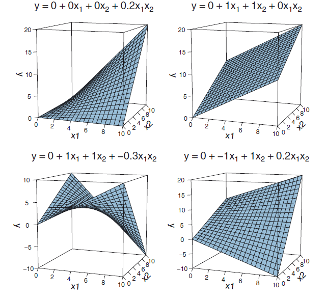
Interaction between two continuous variables
##
## Call:
## lm(formula = read ~ math * socst, data = dSoc)
##
## Residuals:
##      Min       1Q   Median       3Q      Max
## -18.6071  -4.9228  -0.7195   4.5912  21.8592
##
## Coefficients:
##              Estimate Std. Error t value Pr(>|t|)
## (Intercept) 37.842715  14.545210   2.602  0.00998 **
## math        -0.110512   0.291634  -0.379  0.70514
## socst       -0.220044   0.271754  -0.810  0.41908
## math:socst   0.011281   0.005229   2.157  0.03221 *
## ---
## Signif. codes:  0 '***' 0.001 '**' 0.01 '*' 0.05 '.' 0.1 ' ' 1
##
## Residual standard error: 6.96 on 196 degrees of freedom
## Multiple R-squared:  0.5461, Adjusted R-squared:  0.5392
## F-statistic: 78.61 on 3 and 196 DF,  p-value: < 2.2e-16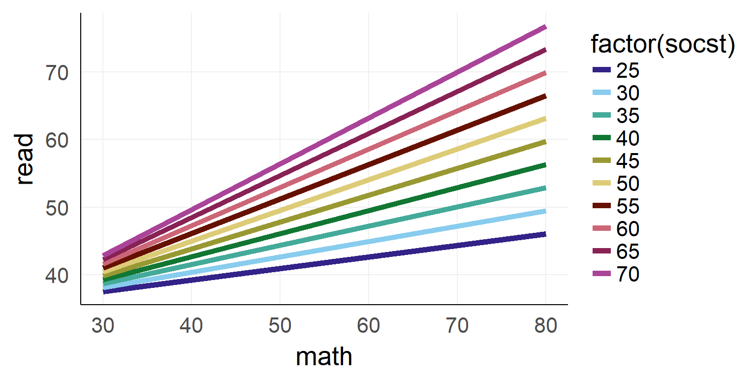
Interaction as a plane
Overview
- Warmup
- Why statistics
- do it yourself statistics
- Linear Regression
- Multiple Regression
- Categorical Variables
- Interactions and the famous 2x2 design
- Inference
- single parameter
- model comparison
- Asumptions
- Bootstrapping
- Four ways of statistics
- Equivalence of traditional tests
Remember: There is only one statistical test
 We need to specify our H0
General assumption for all of the following inference: Independence of residuals
Two general ways
sampling distribution of predictors (walds t-test)
- walds-t = \(\frac{estimate}{SE}\)
- tests a single predictor
- coding scheme influences what is tested (good and bad)
Model comparison / F-test
- Test how well a model with predictor vs. one without explain the data
- Can test sets of predictors at the same time
Generally the two tests will agree in the case of a single predictor to be tested (\((waldsT)^2 = F\)).
This will be not true when we reach GLMs and in multiple regression only for high \(n\)
What is a standard error?
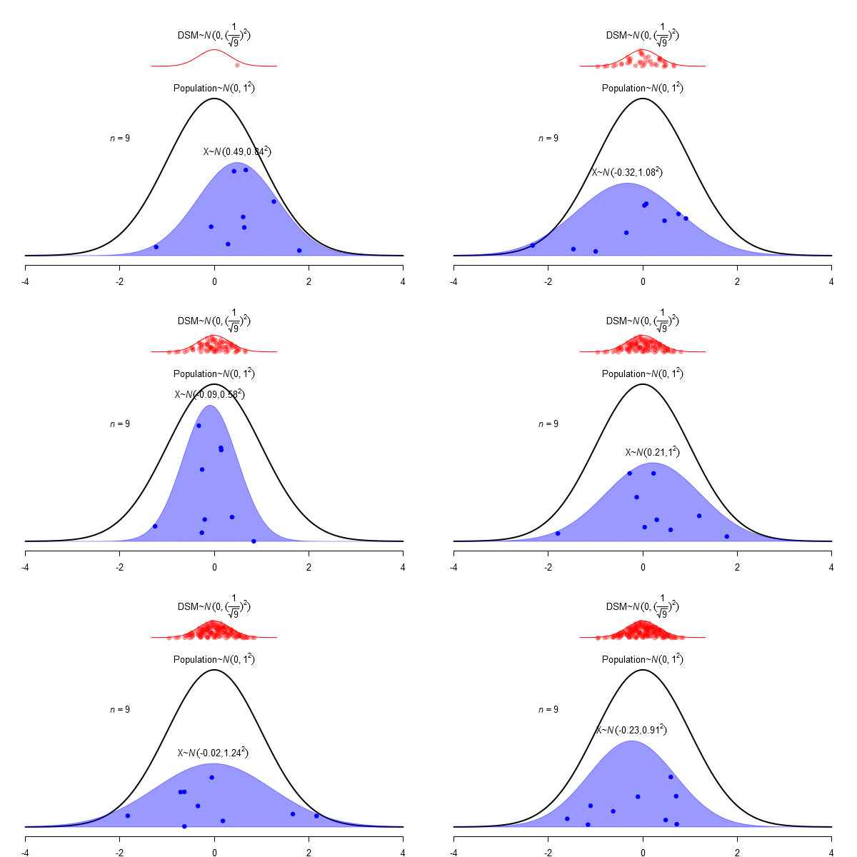
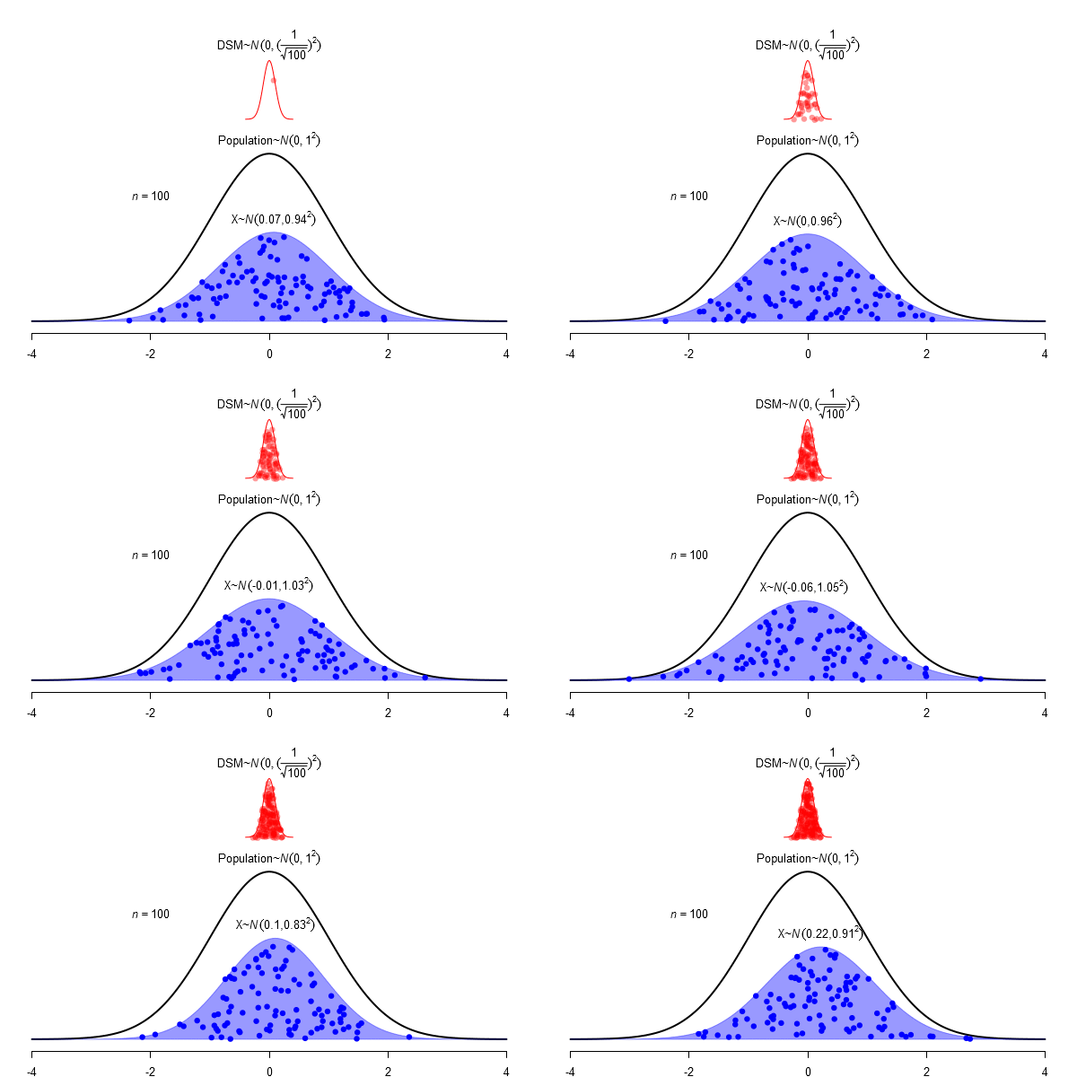
\(SEM = \frac \sigma{\sqrt{N}}\)
Confidence Interval as an area of the sampling distribution
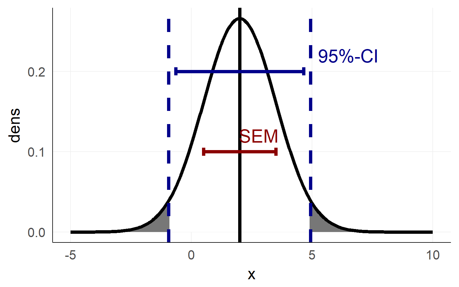
Confidence intervals visualized
Important notes on confidence intervals
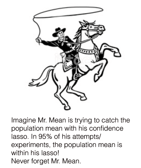
An estimated mean \(\hat \mu\) of a population is either in a proposed range (e.g. confidence interval) or its not.
There is not a 95% probability that the population mean \(\mu\) is in a calculated 95%-confidence interval
The 95% are attached to the confidence-interval NOT the mean
=> 95% of confidence-intervals contain the population mean \(\mu\)
- There is no way of knowing whether your confidence interval contains \(\mu\) :(
Just to be sure: Mr. Mean
The \(H_0\) for the simple regression
\(\mu\) - the mean:
- For the intercept (usually): Intercept = 0
- For the slope (usually): slope = 0
But what is the width of the sampling distribution we should use?
In other words: How does the lm function know what the standard errors (\(\frac{\sigma}{sqrt(n)}\)) are?
Expert slide: Estimating standard errors from X
\(\beta = (X^TX)^{-1}X^Ty\)
\(SE = \sqrt{diag(\sigma^2 (X^TX)^{-1})}\)
Quickly summarized: it looks at partial correlations of X (\(X^TX\) => Covariance, inverse => partial correlations) and weights them with the residuals’ variance \(\hat \sigma\)
Walds t-test
summary(fit)##
## Call:
## lm(formula = read ~ math * socst, data = dSoc)
##
## Residuals:
## Min 1Q Median 3Q Max
## -18.6071 -4.9228 -0.7195 4.5912 21.8592
##
## Coefficients:
## Estimate Std. Error t value Pr(>|t|)
## (Intercept) 37.842715 14.545210 2.602 0.00998 **
## math -0.110512 0.291634 -0.379 0.70514
## socst -0.220044 0.271754 -0.810 0.41908
## math:socst 0.011281 0.005229 2.157 0.03221 *
## ---
## Signif. codes: 0 '***' 0.001 '**' 0.01 '*' 0.05 '.' 0.1 ' ' 1
##
## Residual standard error: 6.96 on 196 degrees of freedom
## Multiple R-squared: 0.5461, Adjusted R-squared: 0.5392
## F-statistic: 78.61 on 3 and 196 DF, p-value: < 2.2e-16\(wald-t = \frac{\beta}{SE}\)
wald-t is not normal distributed but t-distributed
What is a t-distribution?
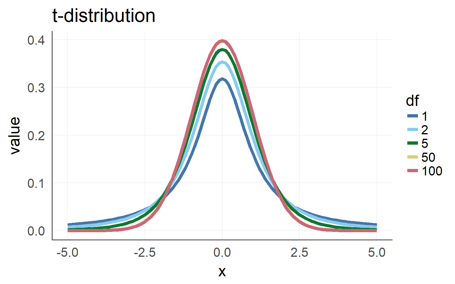
Population \(\sigma\) is unknown. Sampling \(\hat \sigma\) has to be used.
=> Sampling distribution (for small n) is not normal distributed but student t-distributed (with given degrees of freedom)
Overview
- Warmup
- Why statistics
- do it yourself statistics
- Linear Regression
- Multiple Regression
- Categorical Variables
- Interactions and the famous 2x2 design
- Inference
- single parameter
- model comparison
- Asumptions
- Bootstrapping
- Four ways of statistics
- Equivalence of traditional tests
Variance Explained / F-Test
\[R^2 = 1-\frac{var(residual_{full})}{var(residual_{reduced})}\]
In order to get the variance explained of the full/reduced model we need to fit the model twice, once with the effect and once without. Conceptually, the test boils down to:
var1 = var(resid(lm(data=d,hp~1+wt)))
var0 = var(resid(lm(data=d,hp~1)))
r^2  = 1-var1/var0
Empirical distribution:
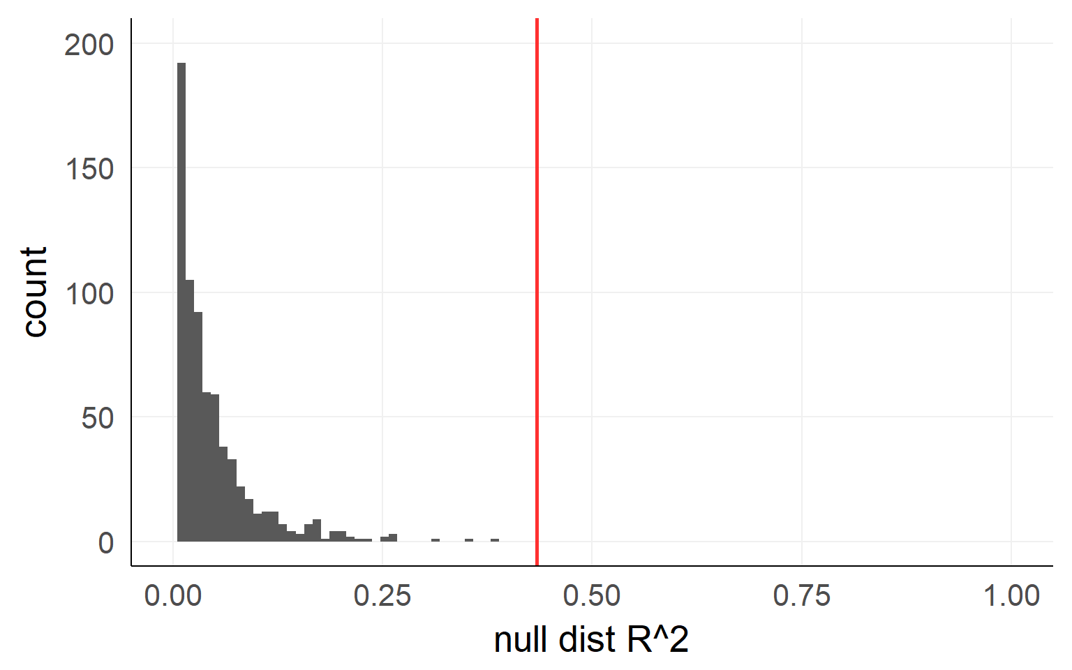
Analytic solution
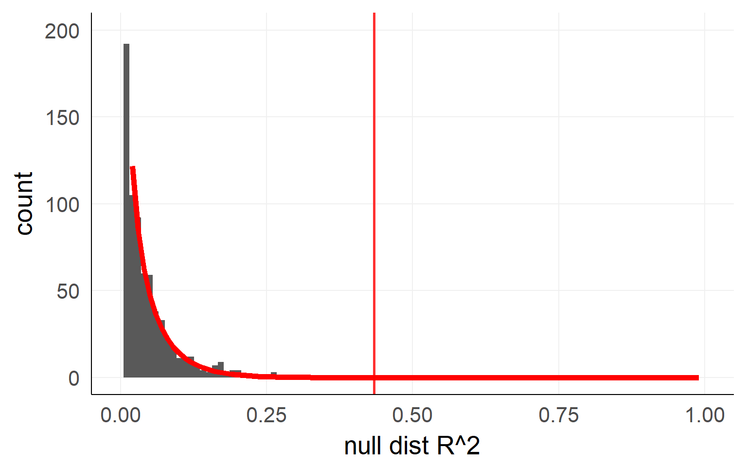
An analytical form is available here as well
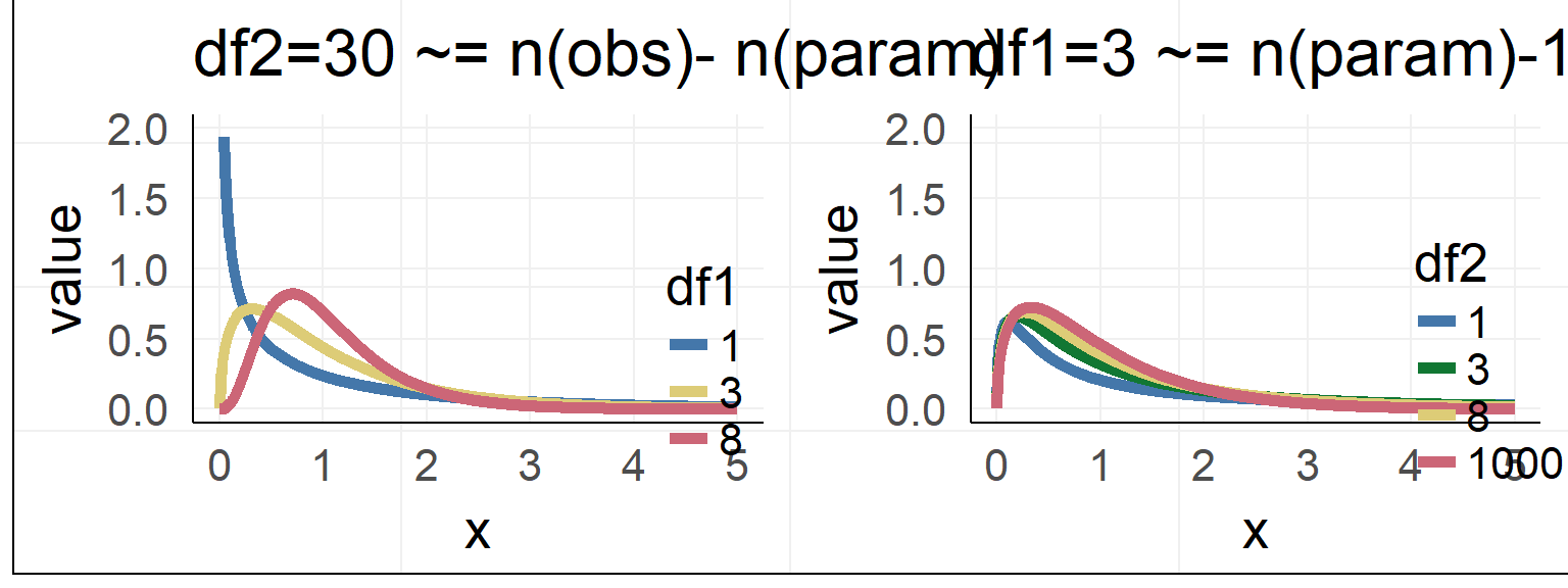
Usually F-distribution is used
\[ F = \frac{\frac{R^2_{m+k}-R^2_{m}}{df_1}}{\frac{1-R^2_{m+k}}{df_2}} = \frac{R^2_{m+k}-R^2_{m}}{1-R^2_{m+k}} * \frac{df_2}{df_1}\] with bookkeeping (for 1xk ANOVA):
\(df_1 = k\), with \(k\) the number of predictors
\(df_2 = n - m - k -1\), with \(n\) the number of observations, \(m\) the number of total predictors
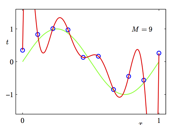
Overfit
var-explained(predictorA) \(<=\) Var-explained(predictorA + predictorB)
Explained-variance is not everything. We also have to take into account the number of predictors we include
Categorical predictor with multiple levels
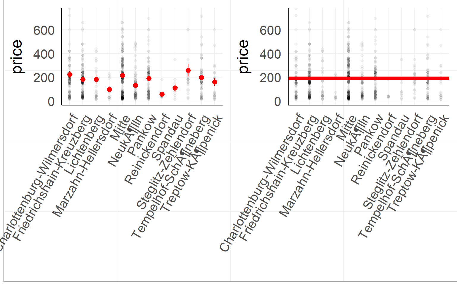
Airbnb prices against location in Berlin (first 900 entries)
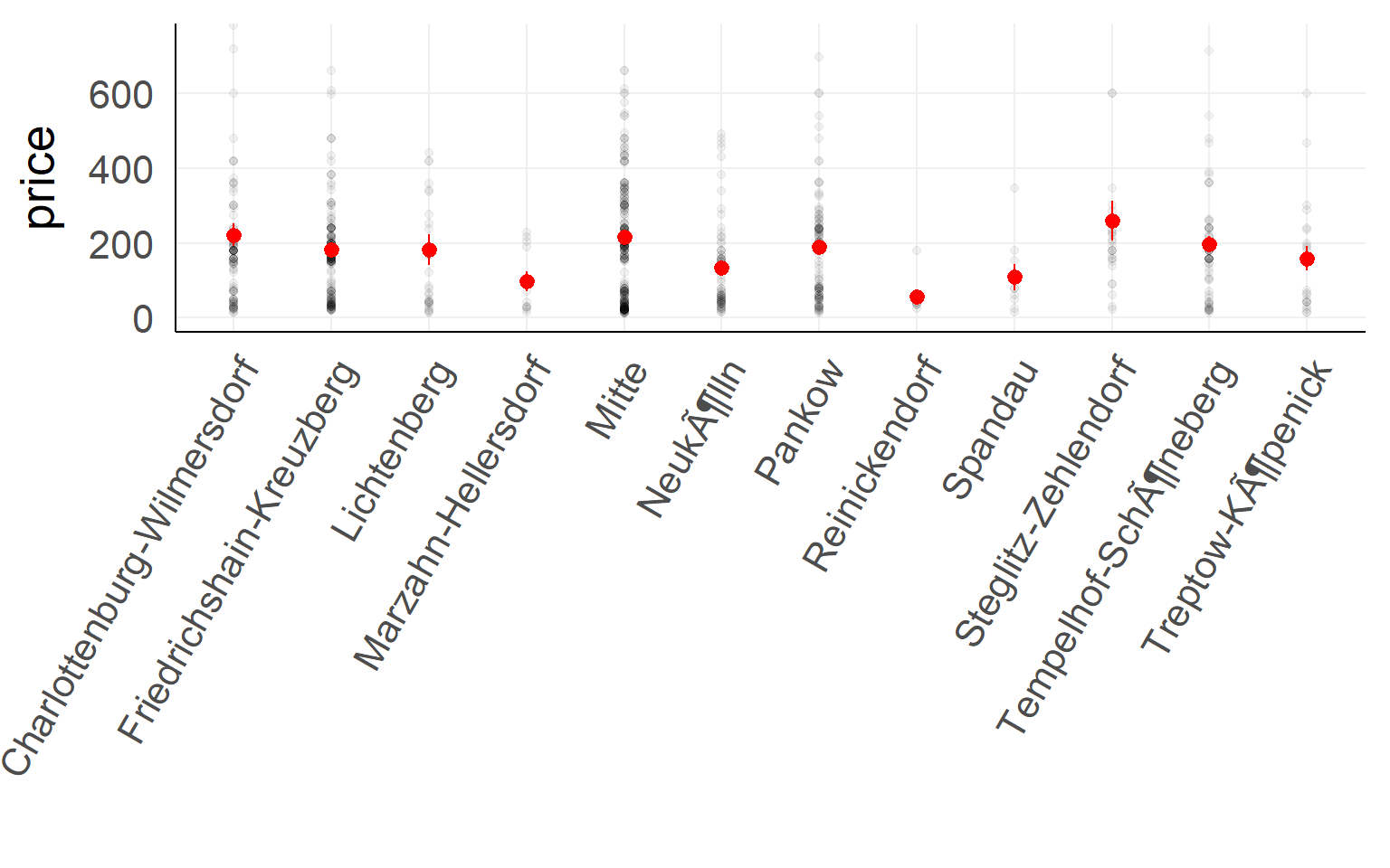
Testing
summary(lm(price~1+ngb,dair[1:900,]))##
## Call:
## lm(formula = price ~ 1 + ngb, data = dair[1:900, ])
##
## Residuals:
## Min 1Q Median 3Q Max
## -237.30 -134.55 -27.47 45.21 2822.60
##
## Coefficients:
## Estimate Std. Error t value Pr(>|t|)
## (Intercept) 222.113 22.833 9.728 <2e-16 ***
## ngbFriedrichshain-Kreuzberg -38.717 28.353 -1.366 0.1724
## ngbLichtenberg -39.647 46.980 -0.844 0.3989
## ngbMarzahn-Hellersdorf -124.022 71.546 -1.733 0.0834 .
## ngbMitte -6.562 26.621 -0.246 0.8054
## ngbNeukölln -89.534 35.416 -2.528 0.0116 *
## ngbPankow -32.324 31.064 -1.041 0.2984
## ngbReinickendorf -166.256 88.011 -1.889 0.0592 .
## ngbSpandau -112.891 78.361 -1.441 0.1500
## ngbSteglitz-Zehlendorf 37.183 48.933 0.760 0.4475
## ngbTempelhof-Schöneberg -24.770 36.215 -0.684 0.4942
## ngbTreptow-Köpenick -62.896 52.155 -1.206 0.2282
## ---
## Signif. codes: 0 '***' 0.001 '**' 0.01 '*' 0.05 '.' 0.1 ' ' 1
##
## Residual standard error: 224.9 on 888 degrees of freedom
## Multiple R-squared: 0.02032, Adjusted R-squared: 0.008188
## F-statistic: 1.675 on 11 and 888 DF, p-value: 0.07433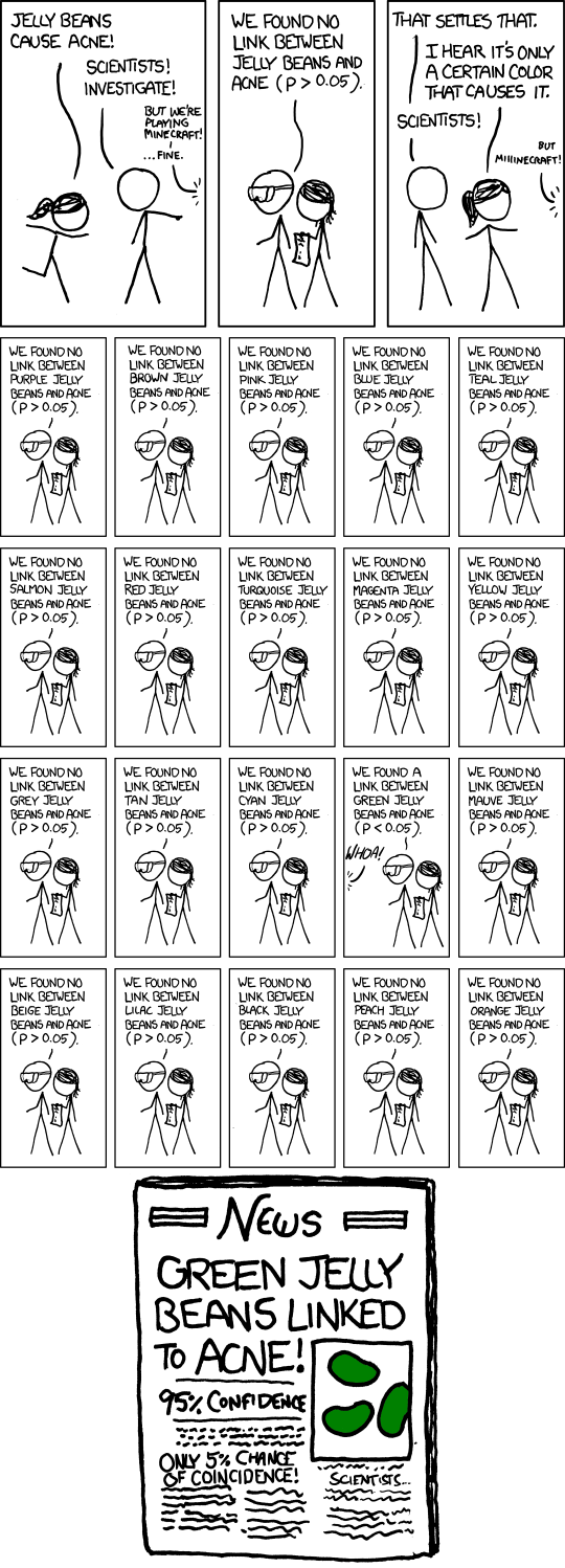
Testing
m0 = lm(price~1    ,dair[1:900,])
m1 = lm(price~1+ngb,dair[1:900,])
anova(m0,m1)
## Analysis of Variance Table
##
## Model 1: price ~ 1
## Model 2: price ~ 1 + ngb
## Res.Df RSS Df Sum of Sq F Pr(>F)
## 1 899 45839663
## 2 888 44908040 11 931623 1.6747 0.07433 .
## ---
## Signif. codes: 0 '***' 0.001 '**' 0.01 '*' 0.05 '.' 0.1 ' ' 1an graphical way to think about it
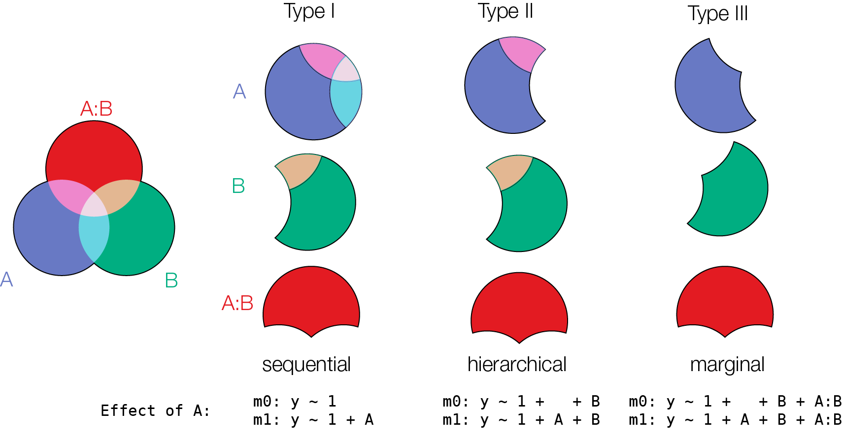
Coming back to a 2x2 design. Which order to test effects?
Model comparison does not care about recoding
##
## Coefficients:
##             Estimate Std. Error t value Pr(>|t|)
## (Intercept)   -17.39      52.44  -0.332  0.74260
## wt             47.14      13.64   3.456  0.00177 **
## am           -123.33      74.03  -1.666  0.10690
## wt:am          63.84      25.08   2.545  0.01672 *
## ---
## Signif. codes:  0 '***' 0.001 '**' 0.01 '*' 0.05 '.' 0.1 ' ' 1
##
## Residual standard error: 44.99 on 28 degrees of freedom
## Multiple R-squared:  0.6111, Adjusted R-squared:  0.5694
## F-statistic: 14.66 on 3 and 28 DF,  p-value: 6.266e-06
##
## Coefficients:
## Estimate Std. Error t value Pr(>|t|)
## (Intercept) -79.06 37.02 -2.136 0.0416 *
## wt 79.06 12.54 6.303 8.12e-07 ***
## am1 -123.33 74.03 -1.666 0.1069
## wt:am1 63.84 25.08 2.545 0.0167 *
## ---
## Signif. codes: 0 '***' 0.001 '**' 0.01 '*' 0.05 '.' 0.1 ' ' 1
##
## Residual standard error: 44.99 on 28 degrees of freedom
## Multiple R-squared: 0.6111, Adjusted R-squared: 0.5694
## F-statistic: 14.66 on 3 and 28 DF, p-value: 6.266e-06Walds-T test cares (simple vs. main effects)
## Analysis of Variance Table
##
## Response: hp
##           Df Sum Sq Mean Sq F value    Pr(>F)
## wt         1  63238   63238 31.2413 5.555e-06 ***
## am         1  12700   12700  6.2744   0.01834 *
## wt:am      1  13111   13111  6.4774   0.01672 *
## Residuals 28  56677    2024
## ---
## Signif. codes:  0 '***' 0.001 '**' 0.01 '*' 0.05 '.' 0.1 ' ' 1
## Analysis of Variance Table
##
## Response: hp
## Df Sum Sq Mean Sq F value Pr(>F)
## wt 1 63238 63238 31.2413 5.555e-06 ***
## am 1 12700 12700 6.2744 0.01834 *
## wt:am 1 13111 13111 6.4774 0.01672 *
## Residuals 28 56677 2024
## ---
## Signif. codes: 0 '***' 0.001 '**' 0.01 '*' 0.05 '.' 0.1 ' ' 1model comparison does not care!
Overview
- Warmup
- Why statistics
- do it yourself statistics
- Linear Regression
- Multiple Regression
- Categorical Variables
- Interactions and the famous 2x2 design
- Inference
- Asumptions
- Bootstrapping
- Four ways of statistics
- Equivalence of traditional tests
- Linearity of responses
- Independence
- Normality
- Equal variance
Linearity of responses
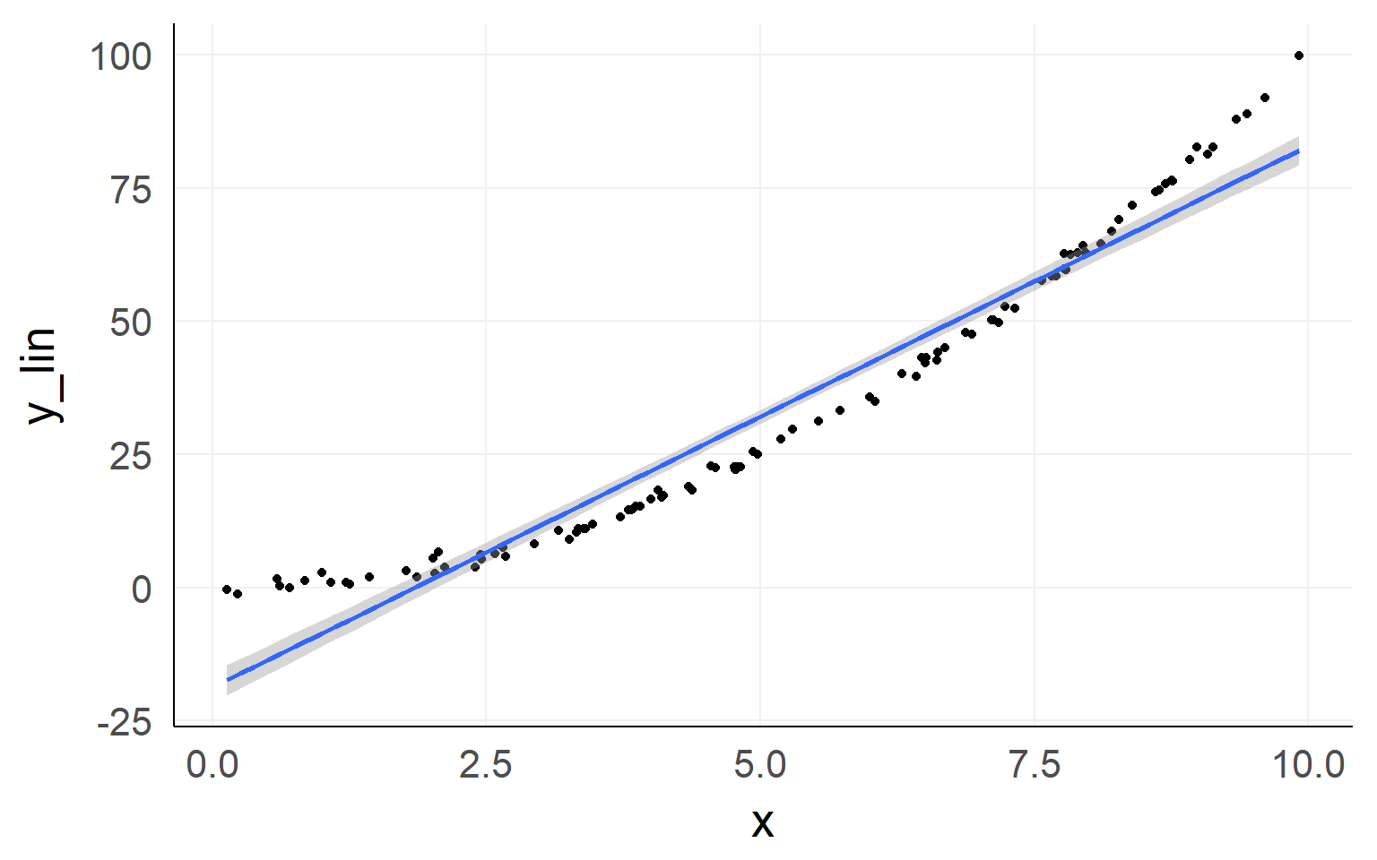
Linear response
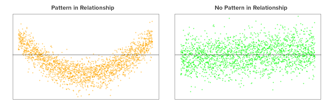
Independence of residuals
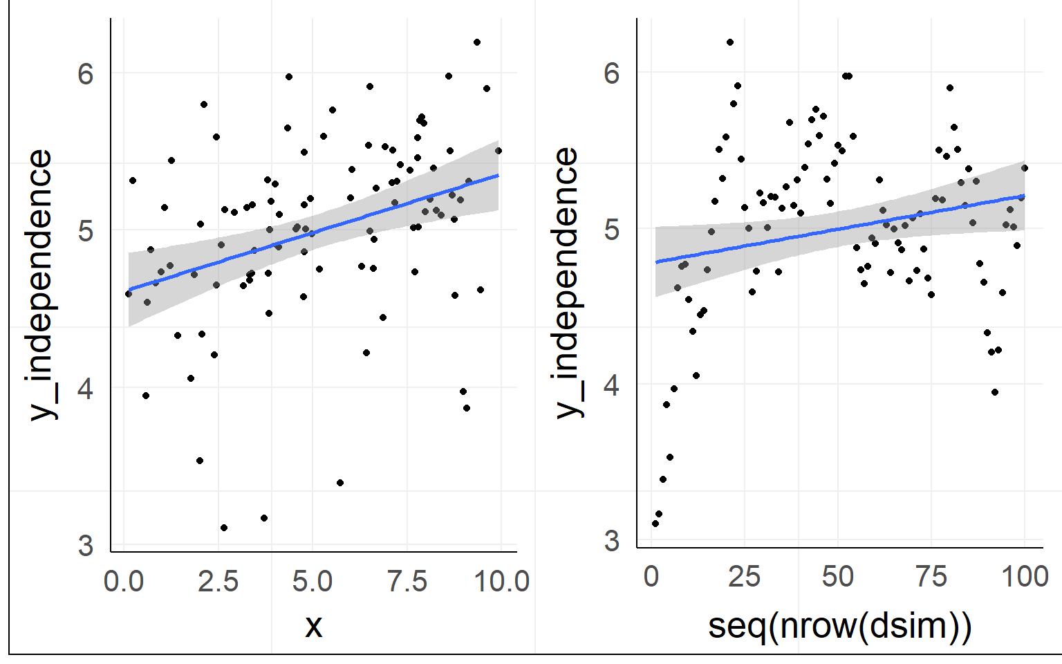
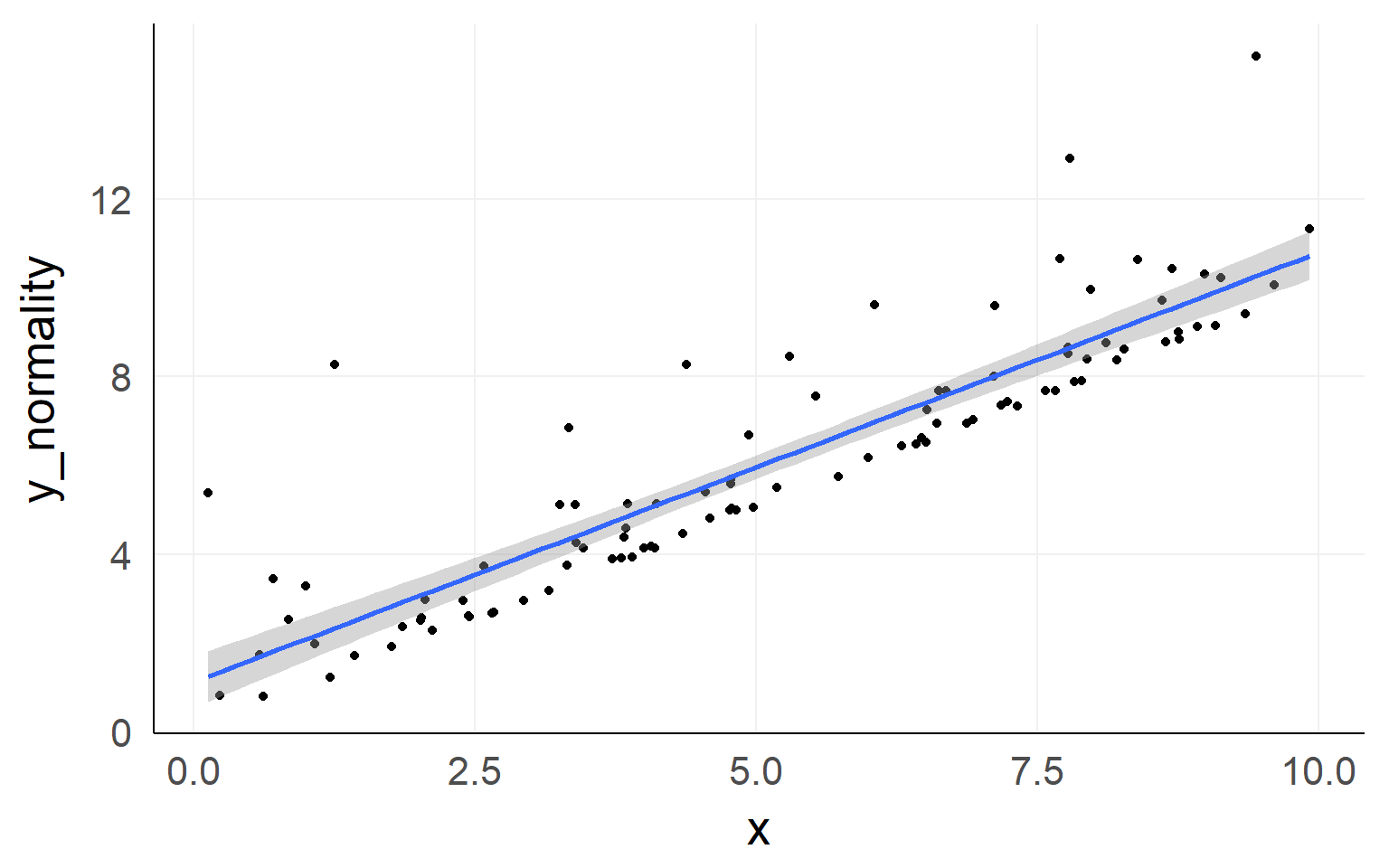
Normality of residuals
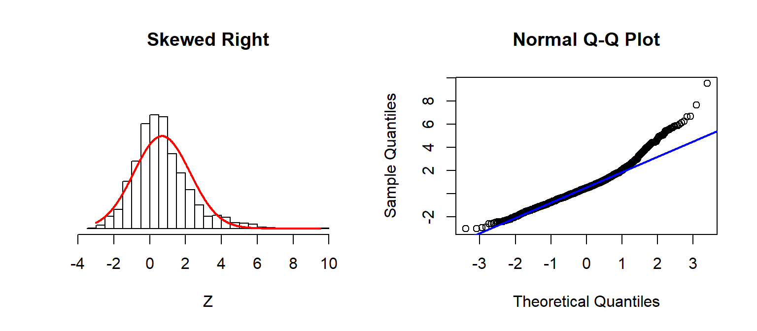
Checking Assumptions: Normality using QQplots
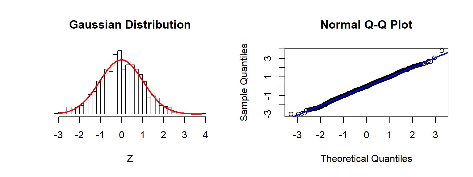
Source: Sean Kross
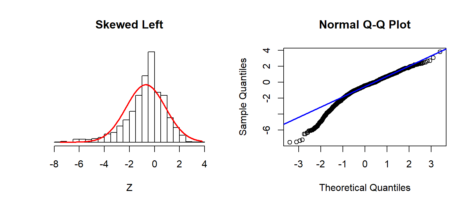
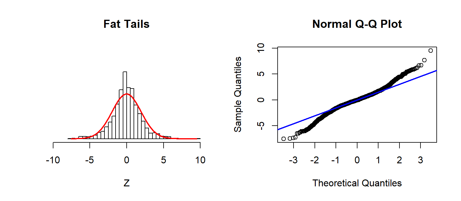
A nice trick
simulate datasets with same specifications and compare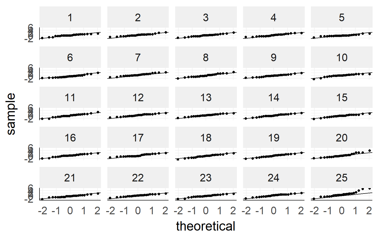
Equal variance

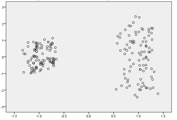
Overview
- Warmup
- Why statistics
- do it yourself statistics
- Linear Regression
- Multiple Regression
- Categorical Variables
- Interactions and the famous 2x2 design
- Inference
- Asumptions
- Bootstrapping
- Four ways of statistics
- Equivalence of traditional tests
A bootstrap visualization
Why bootstrapping?
- Violated assumptions
- Unknown analytical + \(H_0\) distribution
Bootstrap for regression
Bootstrapping in R
##
## Call: lm(formula = read ~ math * socst, data = dSoc)
##              Estimate Std. Error t value Pr(>|t|)
## (Intercept) 37.842715  14.545210   2.602  0.00998 **
## math        -0.110512   0.291634  -0.379  0.70514
## socst       -0.220044   0.271754  -0.810  0.41908
## math:socst   0.011281   0.005229   2.157  0.03221 *
##
## Residual standard error: 6.96 on 196 degrees of freedom
## Multiple R-squared:  0.5461, Adjusted R-squared:  0.5392
## F-statistic: 78.61 on 3 and 196 DF,  p-value: < 1e-04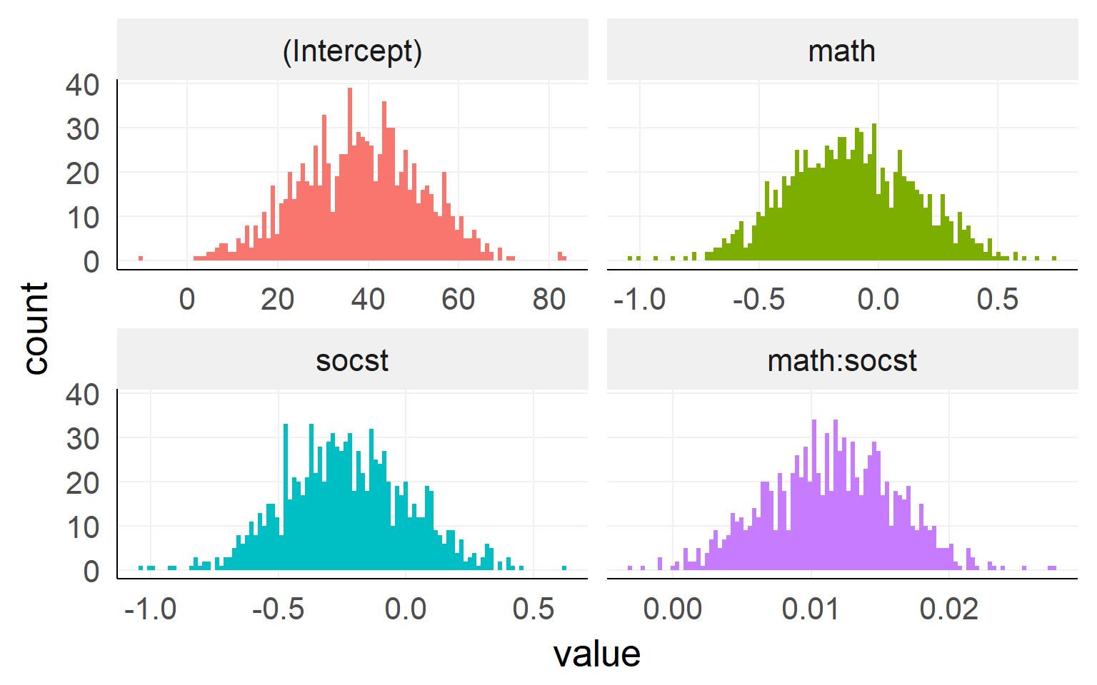
Continued
boot::boot.ci(bootres,type='bca',index=4) # 4 = which parameter from coef to get## BOOTSTRAP CONFIDENCE INTERVAL CALCULATIONS
## Based on 1000 bootstrap replicates
##
## CALL :
## boot::boot.ci(boot.out = bootres, type = "bca", index = 4)
##
## Intervals :
## Level BCa
## 95% ( 0.0018, 0.0196 )
## Calculations and Intervals on Original Scaleconfint(fit,parm = 'math:socst')## 2.5 % 97.5 %
## math:socst 0.0009676529 0.02159379Overview
- Warmup
- Why statistics
- do it yourself statistics
- Linear Regression
- Multiple Regression
- Categorical Variables
- Interactions and the famous 2x2 design
- Inference
- Asumptions
- Bootstrapping
- Four ways of statistics
- Equivalence of traditional tests
- Fisher
- Neyman-Pearson
- NHST (Null Hypothesis Testing)
- Bayes
Fisher
- p-values are a continuous measure of evidence against the \(H_0\)
- “Significant” p-values can be defined ad-hoc, i.e. what you think is enough evidence for this one test
- a sensitivity analysis (~power analysis) can be performed but is not necessary
- General idea: A single experiment should inform your decisions
Neyman-Pearson
- p-values are only used to be threshold by \(\alpha\)
- the pre-analysis fixed \(\alpha\) denotes the error-probability to receive false positives
- a power analysis is required and is part of the test
- a p-value of 0.049 and 0.001 give the same evidence (with \(\alpha=0.05\))
- General idea: Its all about long-term properties. A single experiment does not really help
Type I vs. Type II errors
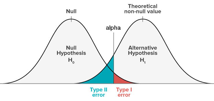
Type Errors

NHST
A dark mix between Fisher & Neyman-Pearson is currently used. This is evident by calculating a p-value, p-values below \(\alpha\) are significant (NP). But exact p-values are still reported.
This is a very popular mix - but is not consistent. Either you want to accept / reject a finding (and be correct on the long run) or you want to identify how much evidence you have from your sample (and act according to how much evidence you have).
Bayes
- parameter estimates (combined with the apropriate aka fully informed prior) reflect the probability of the true parameter being this value
- P-Values are of no use - one can contrast two opposing hypotheses directly (e.g. model-selection)
- usually not interested in testing hypotheses, but more on estimating likely ranges of parameters
An intuition on the difference between Bayes & Frequentist
- Frequentist:
- All about the sampling distribution
- probabilities are frequencies of (hypothetical) outcomes
- Hypothetical Population and experiments (=> sampling distribution)
- A population-parameter has a true value
- “top down”
- Bayesian:
- All about the (subjective*) probabilities of parameters
- probabilities are plausibilities/certainties
- population-parameters are uncertain
- “bottom up”
They can result in exactly the same numbers. But interpretation vastly different!
- sometimes called subjective because of subjective choice of priors
Be both if you can!
Come join our Seminar: “Statistical Rethinking Reading Club” next semester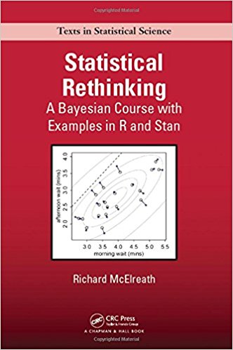
“This is a rare and valuable book that combines readable explanations, computer code, and active learning.” —Andrew Gelman, Columbia University
“…an impressive book that I do not hesitate recommending for prospective data analysts and applied statisticians!” —Christian Robert, Université Paris-Dauphine (review)
“A pedagogical masterpiece…” —Rasmus Bååth, Lund University
“The content of this book has been developed over a decade+ of McElreath’s teaching and mentoring of graduate students, post docs, and other colleagues, and it really shows.” —Brian Wood, Yale
“…omg suddenly everything makes sense…” —Ecstatic anonymous reader
Overview
- Warmup
- Why statistics
- do it yourself statistics
- Linear Regression
- Multiple Regression
- Categorical Variables
- Interactions and the famous 2x2 design
- Inference
- Asumptions
- Bootstrapping
- Four ways of statistics
- Equivalence of traditional tests
Correlation
\[r = \frac{cov_{XY}}{\sigma_X\sigma_Y}\] \[ Y = \beta_0 + X\beta_1\] \[ r = \beta_1\frac{\sigma_X}{\sigma_Y}\]
Alternative: standardize both Y & X (e.g. \(Y^* = \frac{Y}{\sigma_Y}\)) before fitting the regression, you will receive correlations
t-test
Test for two groups: \(t = \frac{\hat \mu_1 - \hat \mu_2}{\sqrt{SE_1^2 + SE_2^2}}\)
t.test(data$DriversKilled[data$law==0],data$DriversKilled[data$law==1],var.equal = T)##
## Two Sample t-test
##
## data: data$DriversKilled[data$law == 0] and data$DriversKilled[data$law == 1]
## t = 4.7942, df = 190, p-value = 3.288e-06
## alternative hypothesis: true difference in means is not equal to 0
## 95 percent confidence interval:
## 15.07239 36.14552
## sample estimates:
## mean of x mean of y
## 125.8698 100.2609print(summary(lm(data=data,DriversKilled~law)),concise=T)##
## Call: lm(formula = DriversKilled ~ law, data = data)
## Estimate Std. Error t value Pr(>|t|)
## (Intercept) 125.870 1.849 68.082 <1e-04 ***
## law -25.609 5.342 -4.794 <1e-04 ***
##
## Residual standard error: 24.03 on 190 degrees of freedom
## Multiple R-squared: 0.1079, Adjusted R-squared: 0.1032
## F-statistic: 22.98 on 1 and 190 DF, p-value: < 1e-04ANOVA
d = data.frame(datasets::mtcars)
d$gear = factor(d$gear)
summary(aov(hp~gear,data=d))
## Df Sum Sq Mean Sq F value Pr(>F)
## gear 2 64213 32106 11.42 0.00022 ***
## Residuals 29 81514 2811
## ---
## Signif. codes: 0 '***' 0.001 '**' 0.01 '*' 0.05 '.' 0.1 ' ' 1l1 = lm(hp~1+gear,data=d)
l0 = lm(hp~1,data=d)
anova(l1,l0)## Analysis of Variance Table
##
## Model 1: hp ~ 1 + gear
## Model 2: hp ~ 1
## Res.Df RSS Df Sum of Sq F Pr(>F)
## 1 29 81514
## 2 31 145727 -2 -64213 11.422 0.0002196 ***
## ---
## Signif. codes: 0 '***' 0.001 '**' 0.01 '*' 0.05 '.' 0.1 ' ' 1ANCOVA
summary(aov(price~factor(bedrooms)+reviews,dair[1:800,]))## Df Sum Sq Mean Sq F value Pr(>F)
## factor(bedrooms) 8 7797765 974721 26.238 <2e-16 ***
## reviews 1 28260 28260 0.761 0.383
## Residuals 790 29347410 37149
## ---
## Signif. codes: 0 '***' 0.001 '**' 0.01 '*' 0.05 '.' 0.1 ' ' 1l1 = lm(price~1+factor(bedrooms)+reviews,data=dair[1:800,])
l0 = lm(price~1+factor(bedrooms),data=dair[1:800,])
anova(l0,l1)## Analysis of Variance Table
##
## Model 1: price ~ 1 + factor(bedrooms)
## Model 2: price ~ 1 + factor(bedrooms) + reviews
## Res.Df RSS Df Sum of Sq F Pr(>F)
## 1 791 29375670
## 2 790 29347410 1 28260 0.7607 0.3834recommendations
I like these books: - Statistical Rethinking - (more math) Advanced Data Analysis from an elemental point view (Cosma Shalizi)
I like these webpages: https://www.flutterbys.com.au/stats/
And thats it!
