Overview
Repeated measures An example to guide you through the steps
The mixed model
Inference
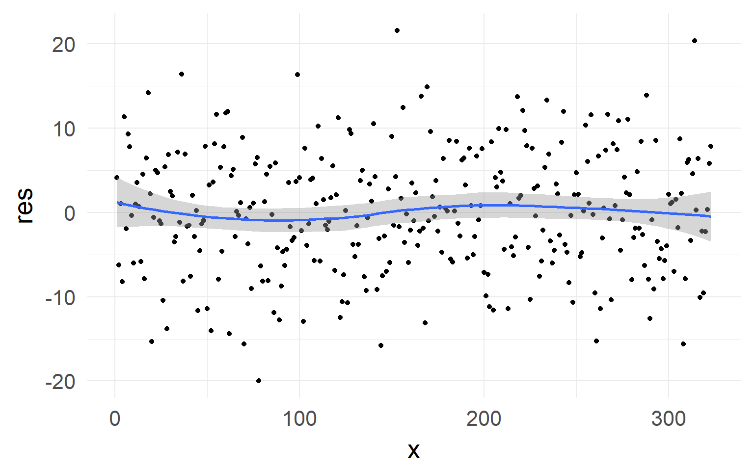
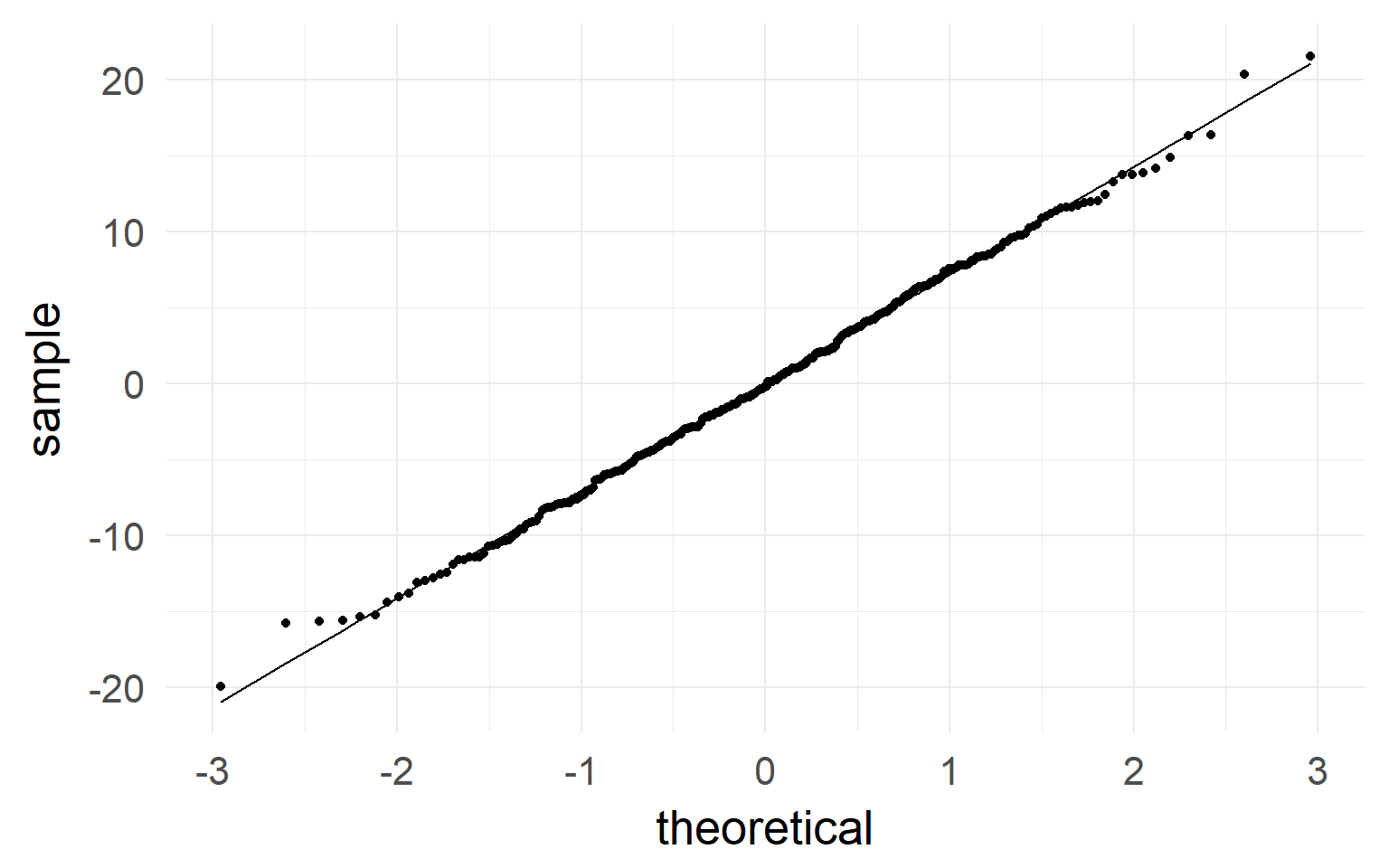
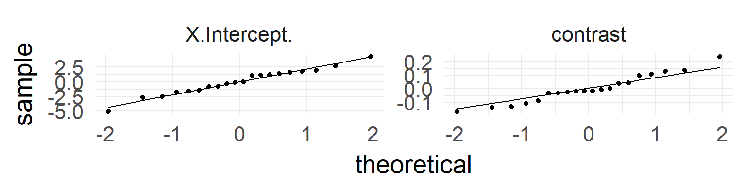
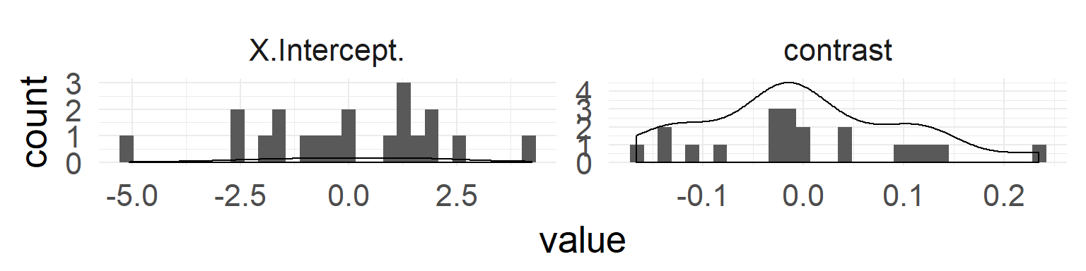
Assumption checking
Shrinkage
Terminology
Convergence Problems
Multiple random variables
Repeated measures
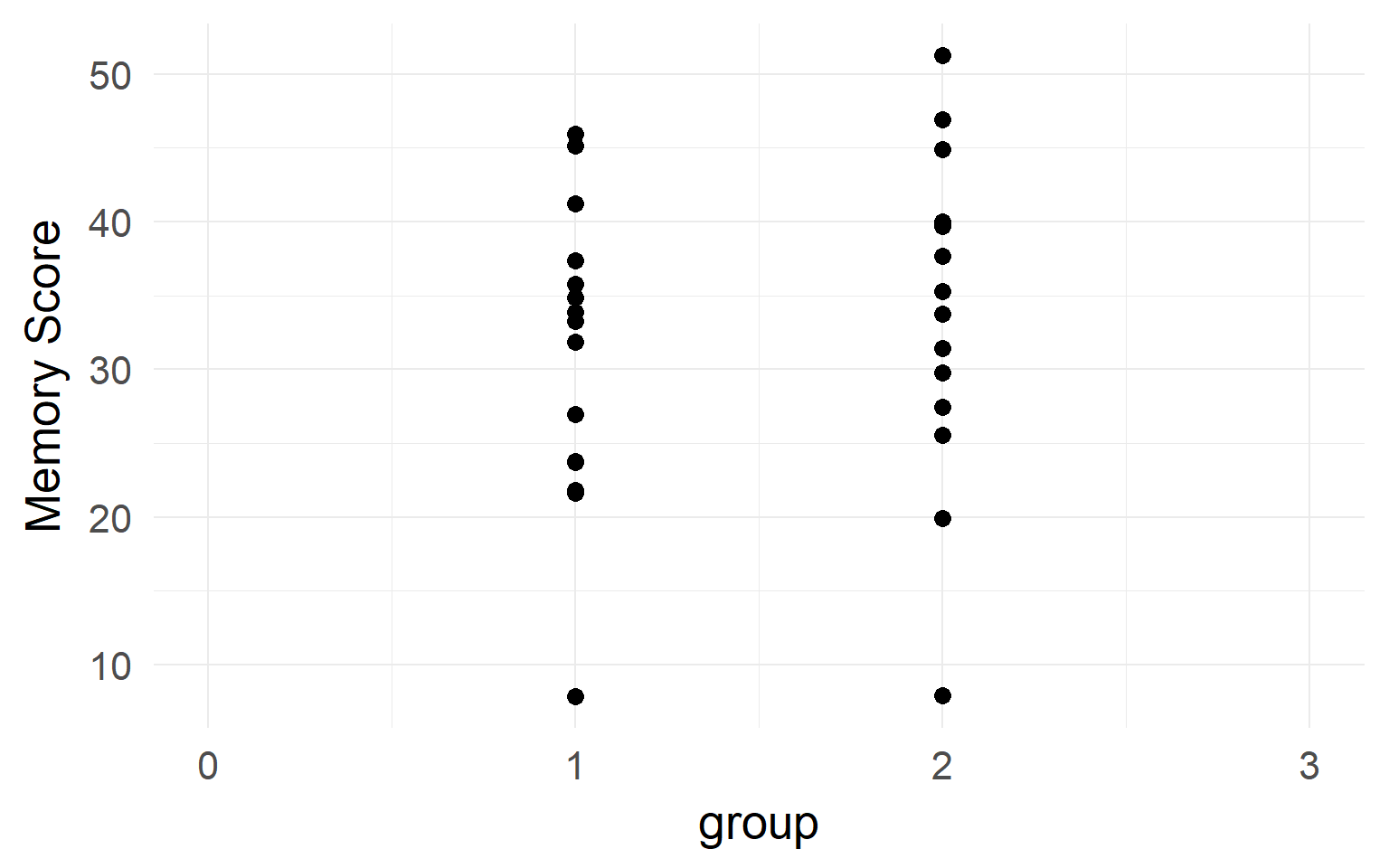
But what if we have data from within the same subjects?
Repeated measures
Each subject is measured in multiple conditions. This allows us to remove individual offsets. Think of an extreme example. One subject has a score in one condition of 1000 and the other condition of 1001. A second subject a score of 10 and 11. The difference between conditions is 1 for both subjects. But if we would assume the data came from four separate subjects, we have to calculate the variance over [10 1000] and [1001 11]. Taking into account repeated measures can remove a lot of distracting effects/variances.
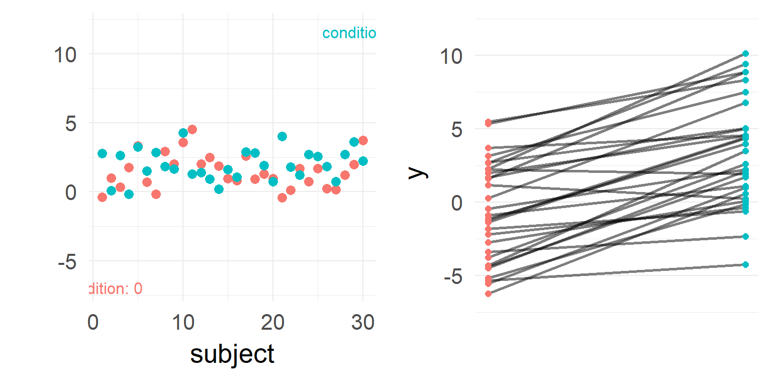
Individual differences
Never analyze repeated measures data without taking repeated measures into account (Disaggregation, Pseudoreplication)
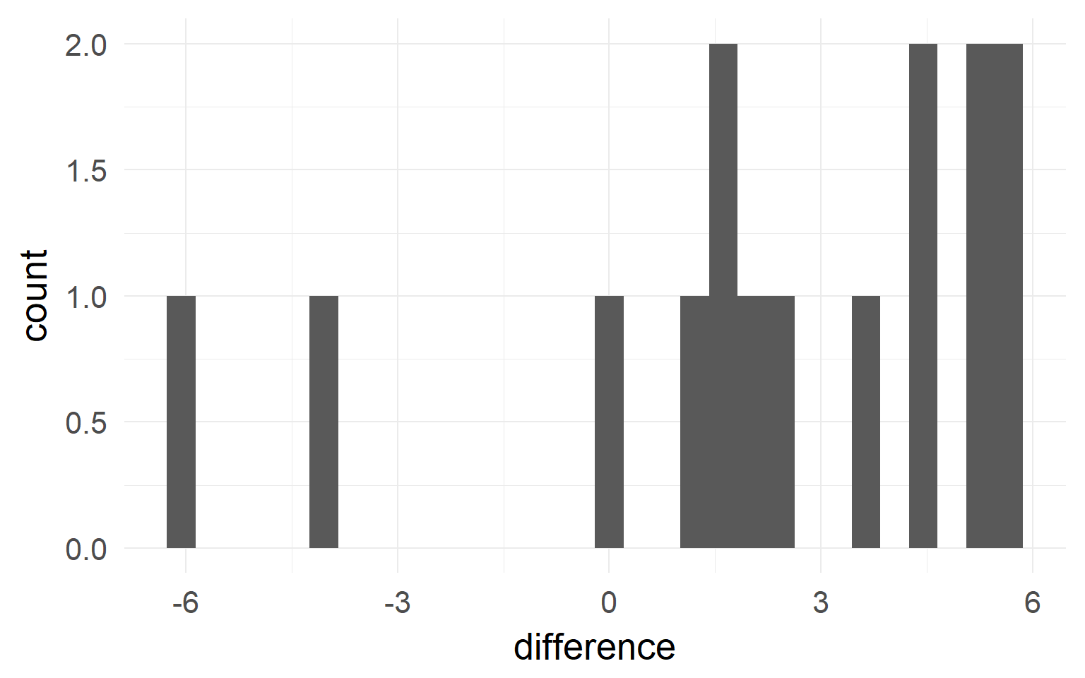
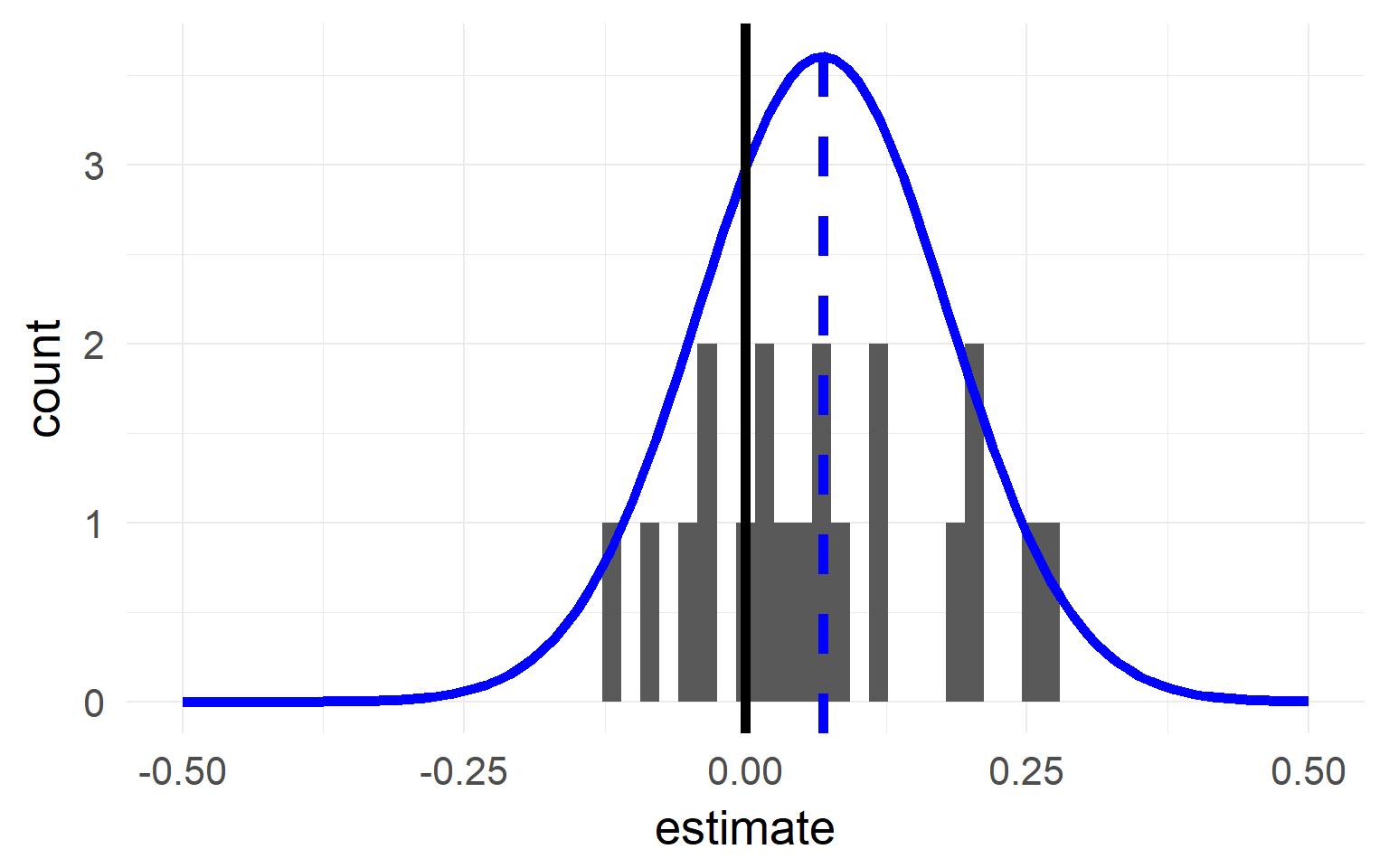
This plot shows the difference, e.g. condition2-condition1 for each subject. This difference values would commonly be tested with a t-test against an assumed \(H_0=0\) . Note that a paired t-test does the same, first calculate the difference and then test this against 0.
Accouting for repeated measures?
\(n_S=5\) subjects
Sampling distributions
The sampling distribution represents the distribution of mean values we would get, if we would repeatedly sample new data (in this case samples with n = 5) from the population. Because we usually do not know the population sample mean, we have to estimate it from our current sample. In this example, we only have 5 data points, thus many population-means seem likely and the sampling distribution is broad.
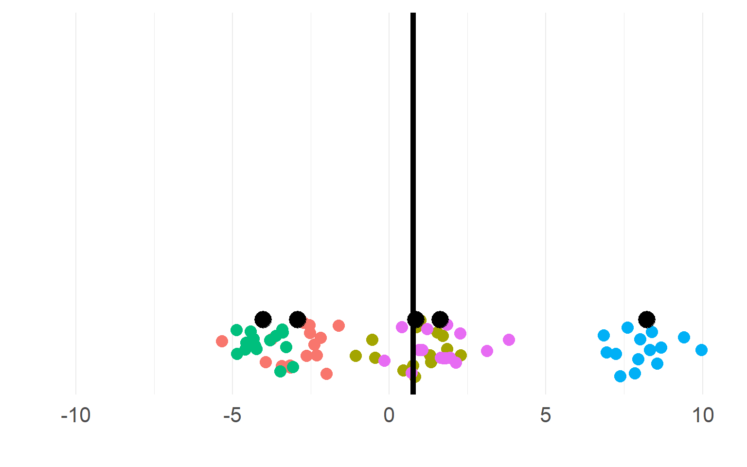
Multiple trials per subject
\(n_T =15\) trials
But what if I tell you that we actually have multiple trials per this black datapoints? Does the situation change?
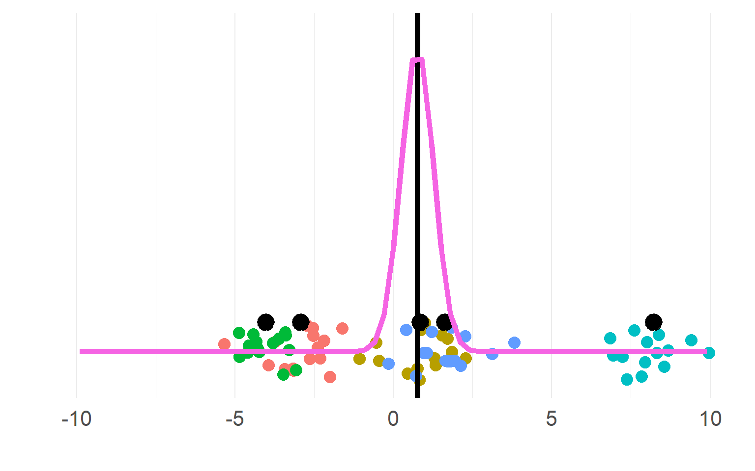
Sampling distributions
The sampling distribution is much smaller now, assumed we forgot that the data arose from the same subjects.
Sampling distributions
(pink for aggregate, purple for disaggregate). There is a strong allure to choose the purple one, easier to get significant results!
\[n_{subject}(aggregate) = df+1 = 5\] \[n_{"subject"}(pseudoreplication) = df+1= 5*5 = 25\]
DONT DO THIS, YOU KNOW (now) BETTER
The \(n_subject\) are interesting because they directly relate to the sampling distribution (\(SE =\frac{\sigma}{\sqrt n}\) ) that is, the higher the estimated number of subjects (or related, degree of freedoms), the smaller the SE, the more “sure” we are.
Taking the student t-test formula, it should become clear, that increasing N, will increase the t-value \(t=\frac{\mu}{\frac{\sigma}{\sqrt n}}\)
Always necessary to aggregate?
\[\sigma_{within} >> \sigma_{between}\]
Subjects are very similar
Not so necessary to aggregate first
A single parameter summarizes subject-means well
\[\sigma_{within} << \sigma_{between}\]
Subjects are very different
Totally necessary to aggregate first
\(n_{subject}\) parameters summarizes subject-means well
’
If all subjects are equal, e.g. you record a dice-throw of each number, you can forget about which subject threw which dice. That is, the variance subjects generate is much smaller than the variance of the outcome.
If subjects are quite different, you have to include this in your analysis. Mixed models are one way to account for the dependency/clusteredness of some measurements (dependency, because knowing 90% of samples of a single subject will inform you on the last 10% of that subject, but not as much of the other subjects, stronger in the “subjects are different” case)
Should we trust all subjects equally?
Question: Estimate the mean of the population
Subjects with high variance might be less reliable. Think of the sampling distribution. For the last subject, the sampling distribution of the mean is probably quite large, the mean of each sample could vary a lot. Maybe one should put less weight on that subject. The first subject has a small variance, the width of the sampling distribution now is small (because the sample-estimate of \(\sigma\) is small \(SE = \frac{\sigma}{\sqrt n}\) ). If we would invite the first subject again, we could be more sure, that the mean would be close to the old mean than for the last subject.
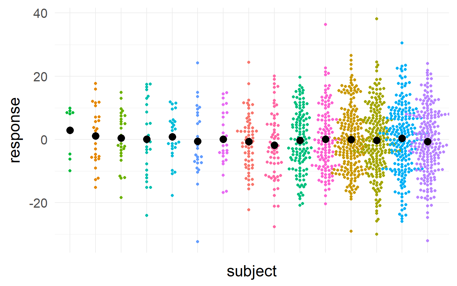
Should we trust all subjects equally?
Question: Estimate the mean of the population
This is a very similar case, but now we do not change \(\sigma\) but \(n\) , the number of samples for each subject. Again think of the sampling distribution. In this case the first subjects will show a broad sampling distribution and should not be weighted as much, the last subjects should show a small distribution and should be weighted more
Should we trust all subjects equally?
We should take into account sample-size and variance into our estimate of the population mean
We should trust those subjects more, where we most sure about their central tendency
Summary
Why repeated measures
More power to find effects that exist!
Don’t forget about repeated measures!
Else your type I error will be very high
Should we trust all subjects equally?
No, we should punish for small within-subject sample-size and punish high variance
At this point it should be said, that this dependency is NOT special to subjects. Imagine you measure how well different classes of a school do. Now agian, you have dependent measures because you can test in each class multiple times (because there are students in there). The first conclusion is that dependencies can arise from many different things. usually it is helpful to think hierarchical. The school example could be increase in both dimensions: Questions - Students - Class - School - District - Nation etc. We will soon learn how to incorporate all this knowledge in the model.
A second point is, repeated measures allow us to remove variance which is great! But standard approaches do not work anymore and might make us TOO confident. Nevertheless if the experimental design allows it, always try to do repeated measures.
Overview
Repeated measures
An example to guide you through the steps
The mixed model Inference
Assumption checking
Shrinkage
Terminology
Convergence Problems
Multiple random variables
A word of warning
Encouraging psycholinguists to use linear mixed-effects models ‘was like giving shotguns to toddlers’ (Barr)
Because mixed models are more complex and more flexible than the general linear model, the potential for confusion and errors is higher (Hamer)
Many ongoing riddles:
Book:Richly Parameterized Linear Models
Chp. 9: Puzzles from Analyzing Real Data sets
Chp.10: A Random Effect Competing with a Fixed Effect
Chp.12: Competition between Random Effects
Chp.14: Mysterious, Inconvenient or Wrong Results from Real Datasets
Mixed models can be complicated. I always try to draw the relation between parameters and explicitly write down the \(y = \beta_0 + \beta_1*X ...\) formula. The link to the book serves just as an example that there can be many strange things going on when doing hierarchical models.
The mixed model in R
\(\hat{y} = \beta_0 + \beta_1 * contrast + u_{0,j} + u_{1,j} * contrast\)
\(\hat{y}_j = \beta X_j + b_jZ\)
Fitting this in R using the package lme4
response ~ beta + (beta|group)
In our example :
response ~ 1 + contrast + (1|subject) + (0+contrast|subject)
Everything in brackets defines that it is nested in the grouping variable. For example (0+contrast|subject) means that contrast is nested in the grouping variable subject. But of course (0+contrast|school) or (0+contrast|image) could be groupings as well. Note that the 0+contrast is necessary and it will be later obvious why.
Mixed models in R
summary (lmer (p100~ 1 + contrast + (1 + contrast|| subject),data= d))## Linear mixed model fit by REML ['lmerMod']
## Formula: p100 ~ 1 + contrast + ((1 | subject) + (0 + contrast | subject))
## Data: d
##
## REML criterion at convergence: 2271.4
##
## Scaled residuals:
## Min 1Q Median 3Q Max
## -2.71978 -0.62658 -0.01064 0.65739 2.91110
##
## Random effects:
## Groups Name Variance Std.Dev.
## subject (Intercept) 10.16741 3.1886
## subject.1 contrast 0.01353 0.1163
## Residual 54.45510 7.3794
## Number of obs: 323, groups: subject, 20
##
## Fixed effects:
## Estimate Std. Error t value
## (Intercept) 4.03422 1.10536 3.650
## contrast 0.09536 0.03045 3.131
##
## Correlation of Fixed Effects:
## (Intr)
## contrast -0.324
This is the model summary output. The important bits are under “Random effects” and “Fixed effects”. Random effects describes the variance component, fixed effects the mean components. We are usually interested in the “fixed effect” estimates (more to the names later). I.e. it is not so interesting how much subjects vary in their mean-effects, but on how large the effect is on average
(1 + contrast||subject) is equal to (1|subject) + (0+contrast|subject)
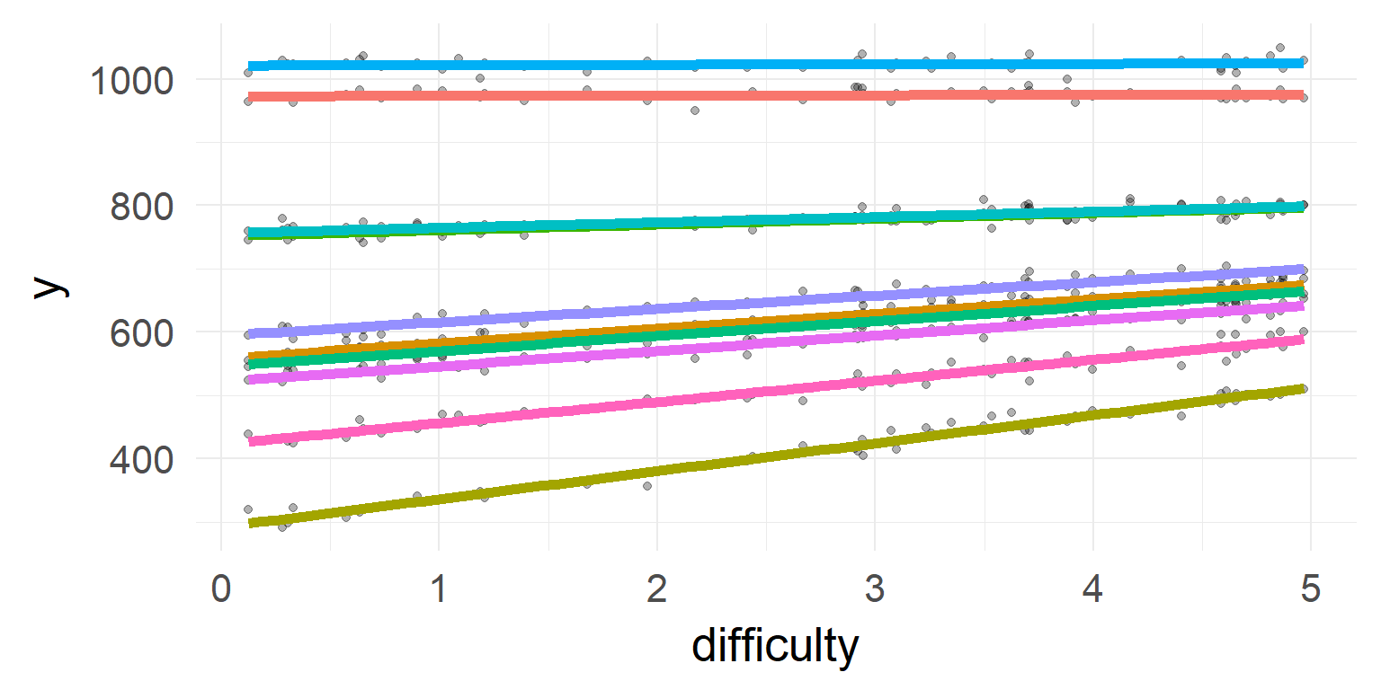
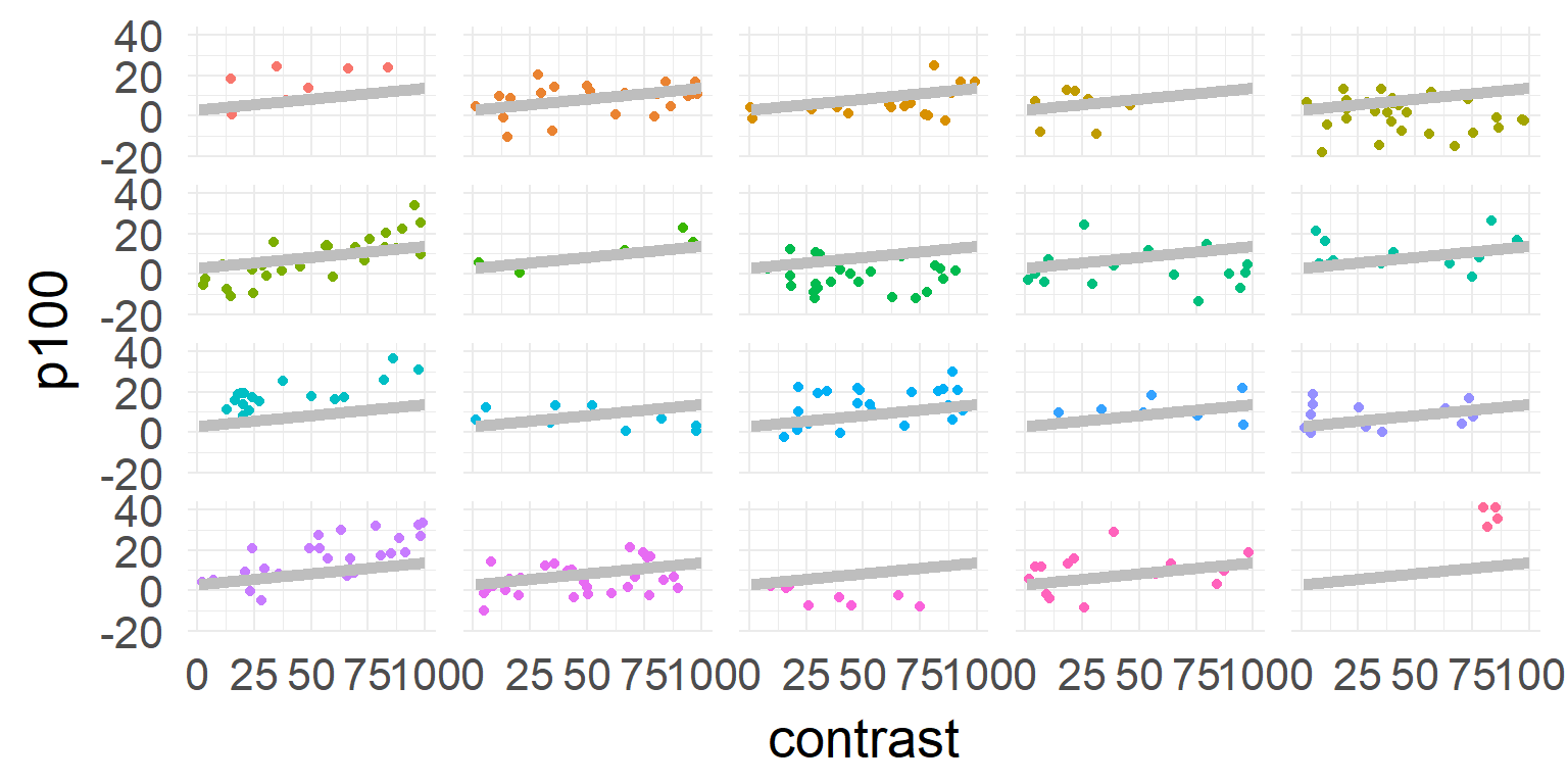
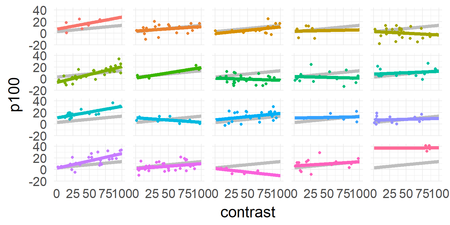
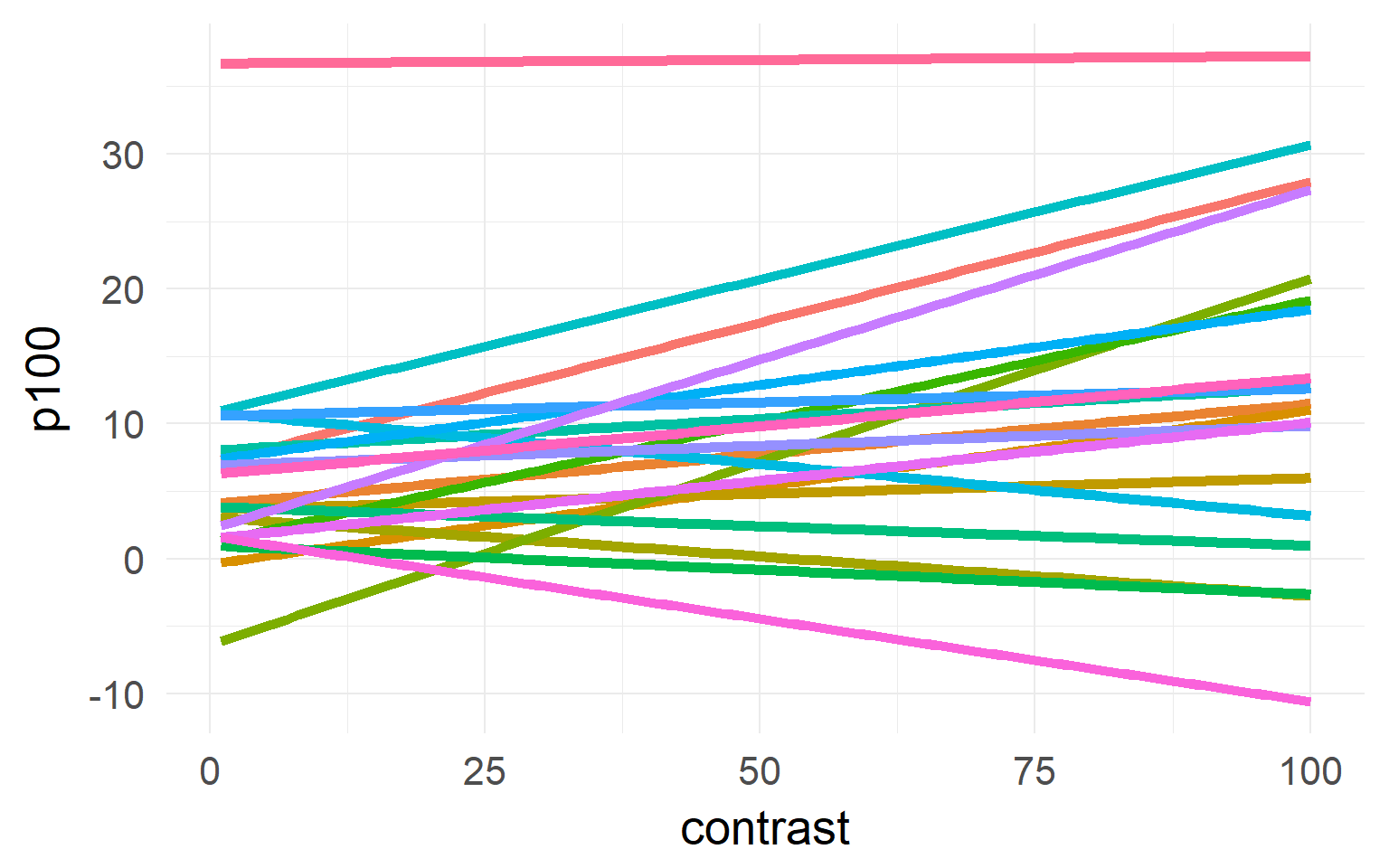
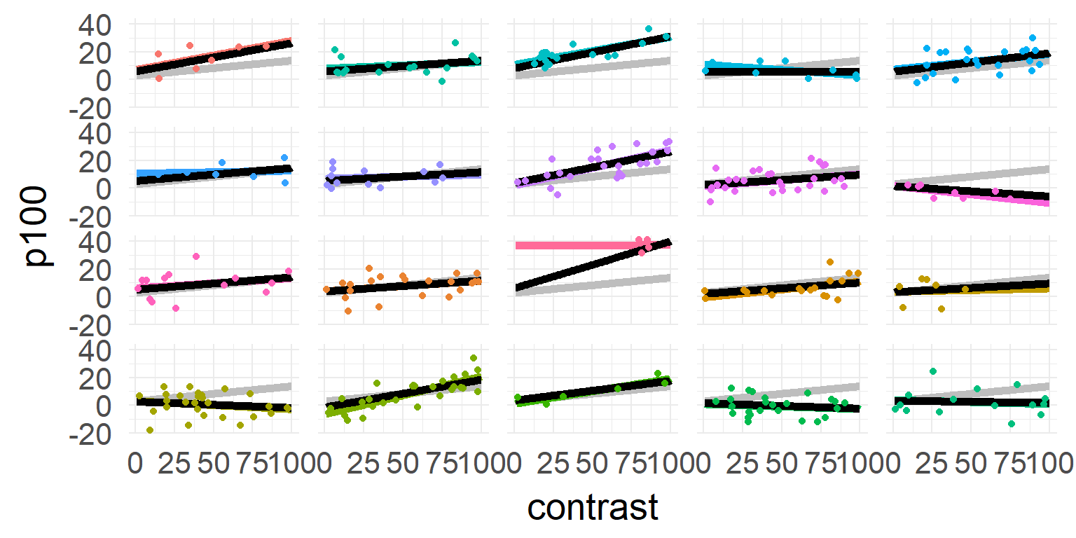
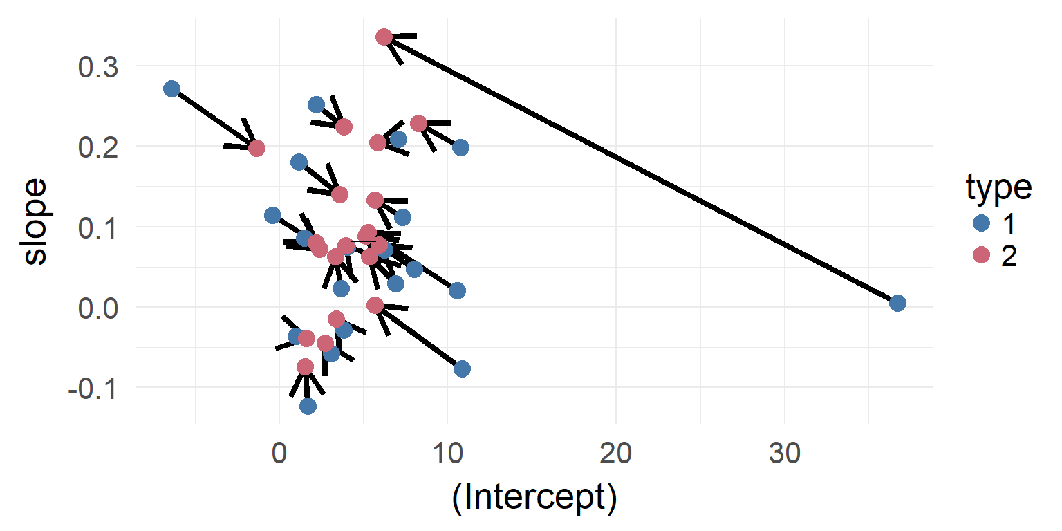
gray: one model, color: individual model, black: mixed model
In our example, we see that the extreme results are not there anymore. For each subject a compromise was build between the average response and their individual ones.
Overview
Repeated measures
An example to guide you through the steps
The mixed model
Inference
Assumption checking
Shrinkage
Terminology
Convergence Problems
Multiple random variables
Model-Comparisons aka p-values
Unresolved problem!
Read (three links):how to get p values , problems with stepwise regression , different ways to get p-values
One way (good and common, but not the best*): Model comparison for fixed effects:
Be sure to keep random structure equal
“refitting model(s) with ML (instead of REML)”
## Data: d
## Models:
## mres0: p100 ~ 1 + (1 + contrast | subject)
## mres1: p100 ~ 1 + contrast + (1 + contrast | subject)
##       Df    AIC    BIC  logLik deviance  Chisq Chi Df Pr(>Chisq)
## mres0  5 2286.5 2305.3 -1138.2   2276.5
## mres1  6 2280.1 2302.7 -1134.0   2268.1 8.4095      1   0.003733 **
## ---
## Signif. codes:  0 '***' 0.001 '**' 0.01 '*' 0.05 '.' 0.1 ' ' 1
* currently bootstrapping or mcmc recommended
In order to check whether a certain parameter/term leads to a better model fit, we can compare two models: One with that parameter (could be a fixed effect or random effect) and one without. The R-anova function performs a likelihood-ratio test. We know from earlier lectures that the outcome of a likelihood ratio test punishes for more parameters, assumed everything is normal distributed, we can look up a probability that adding a parameter with no relation to the data will improve our model as much as the model got improved.
REML VS ML
Intuition:
When estimating the variance parameter using maximum likelihood (ML ) \(\sigma\) is biased because \(\mu\) is not known at the same time
Solution:
Fit all fixed effects \(\mu\) , then refit the variance parameters on the residing estimates.
This is called restricted maximum likelihood (REML ). If \(n\) is large, no difference between ML and REML exist. If \(n\) is small REML gives better predictive results.
ML
For further details see Zuur 2009 (“Mixed Effects Models and Extensions in Ecology with R”, page 116). In practice you do not need to worry too much about the difference. The R anova function will automatically refit your model, if you accidentally used REML instead of ML.
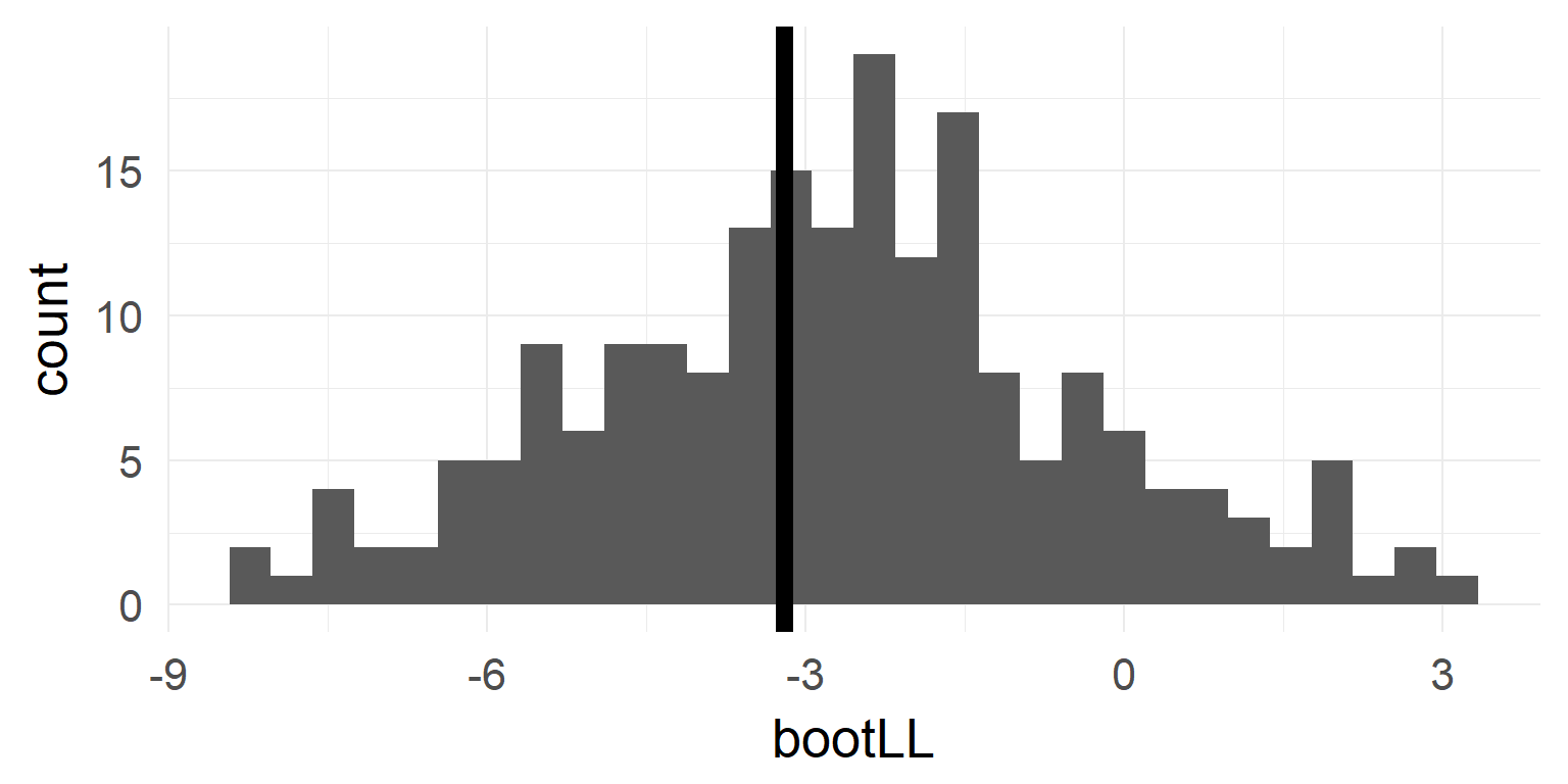
Bootstrapping
resample from the data with replacement (or parametrically from \(H_0\) -Model) 1000 times
calculate statistic of interest
observe spread of statistic
b1 <- bootMer (mres1, FUN = function (x) as.numeric (logLik (x)), nsim = nboot,seed = 1 )
b2 <- bootMer (mres0, FUN = function (x) as.numeric (logLik (x)), nsim = nboot,seed = 1 )
bootLL = 2 * b1$ t - 2 * b2$ t # grab the values & plot
quantile (bootLL, probs = c (0.025 , 0.975 ))
Bootstrapping is a really nice tool. If I would not use Bayes, I would use bootstrapping. The downside is, that its computationally very expensive.
pbkrtest
Better & easier: Likelihood-Ratio using R-Package pbkrtest
summary (pbkrtest:: PBmodcomp (mres1,mres0,nsim= nboot))## Parametric bootstrap test; time: 30.27 sec; samples: 200 extremes: 3;
## large : p100 ~ 1 + contrast + (1 + contrast | subject)
## small : p100 ~ 1 + (1 + contrast | subject)
## stat df ddf p.value
## PBtest 8.3917 0.019900 *
## Gamma 8.3917 0.011404 *
## Bartlett 7.0365 1.0000 0.007986 **
## F 8.3917 1.0000 12.385 0.013029 *
## LRT 8.3917 1.0000 0.003769 **
## ---
## Signif. codes: 0 '***' 0.001 '**' 0.01 '*' 0.05 '.' 0.1 ' ' 1The main con against bootstrapping is the high computational time (use at least 1000 not 200 as in this example)
The book from Phillip Good: “Permutation, Parametric and Bootstrap Tests of Hypotheses” might be a good start to learn more. There are plenty of tutorials out there.
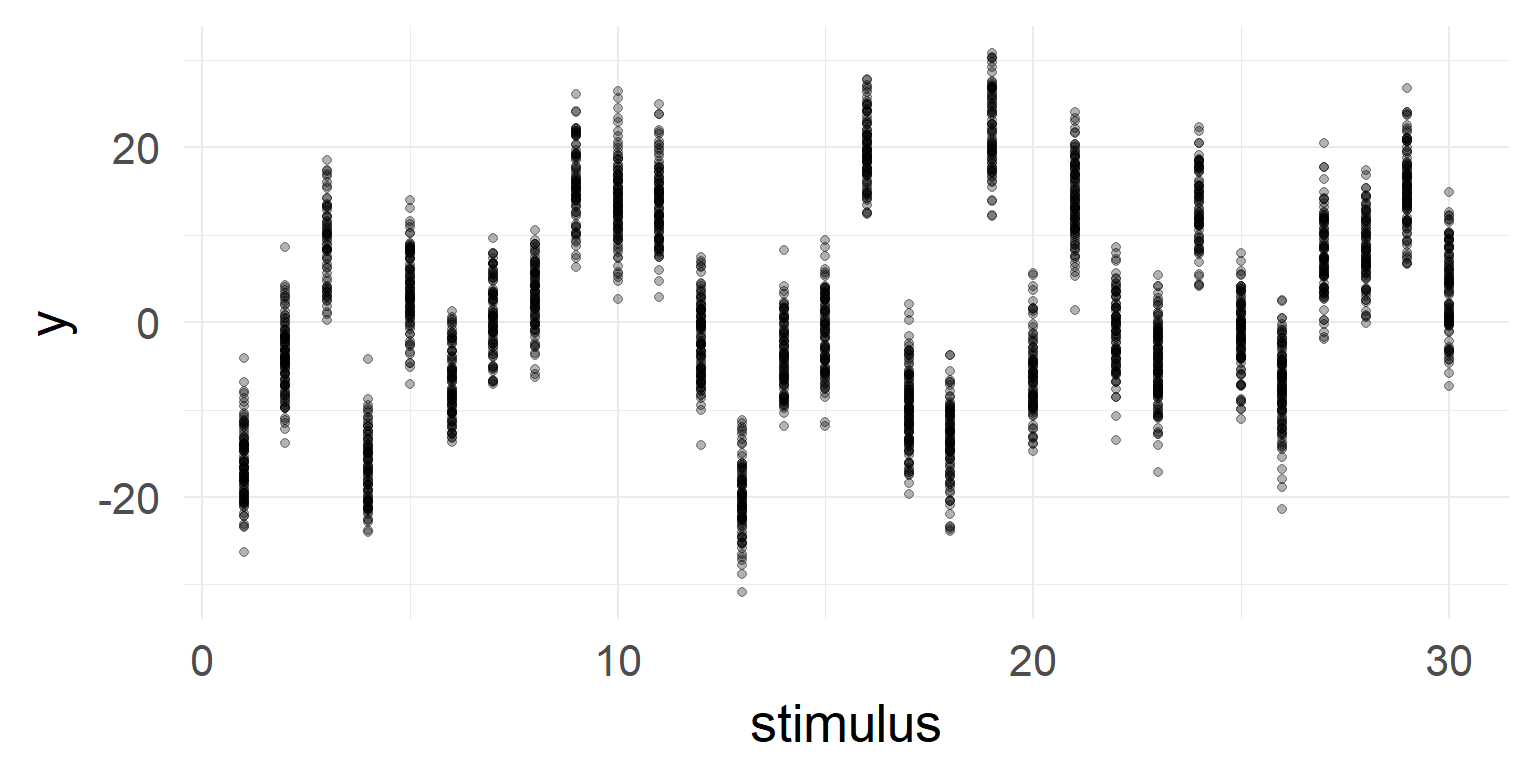
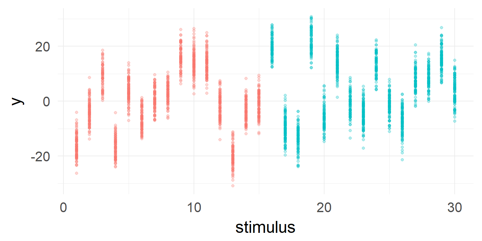
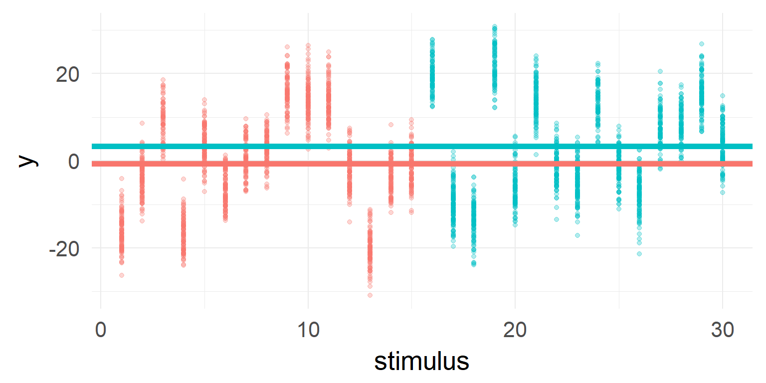
 It looks like there is no difference between groups?
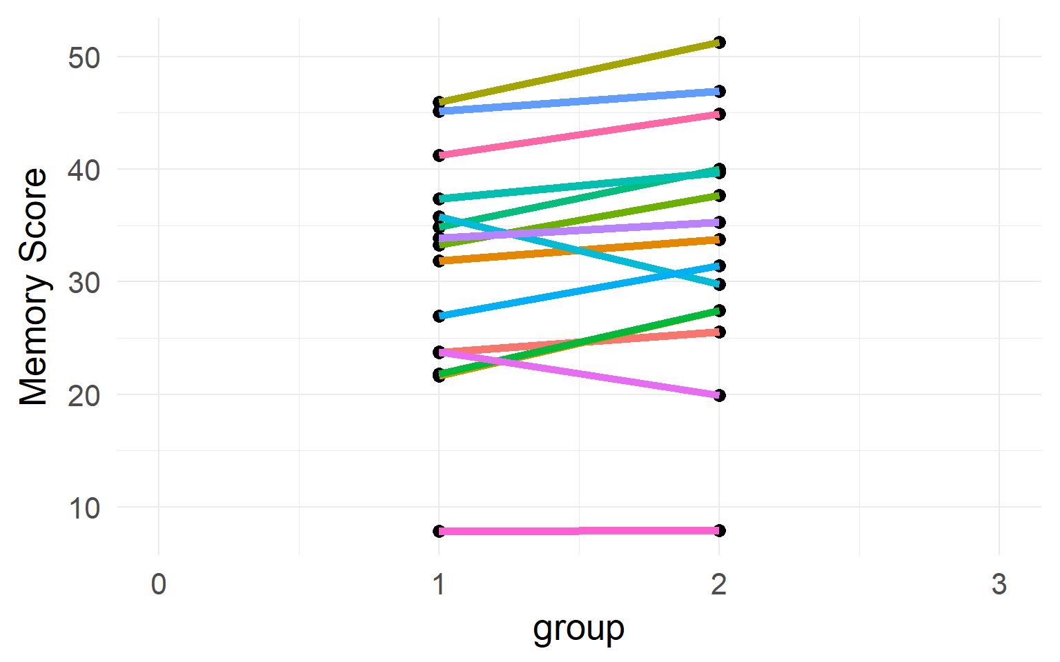
 Between-Subject variability can be removed by repeated measures.
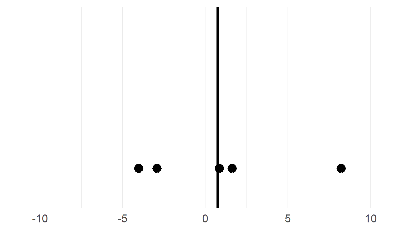 Black = mean of the subject.
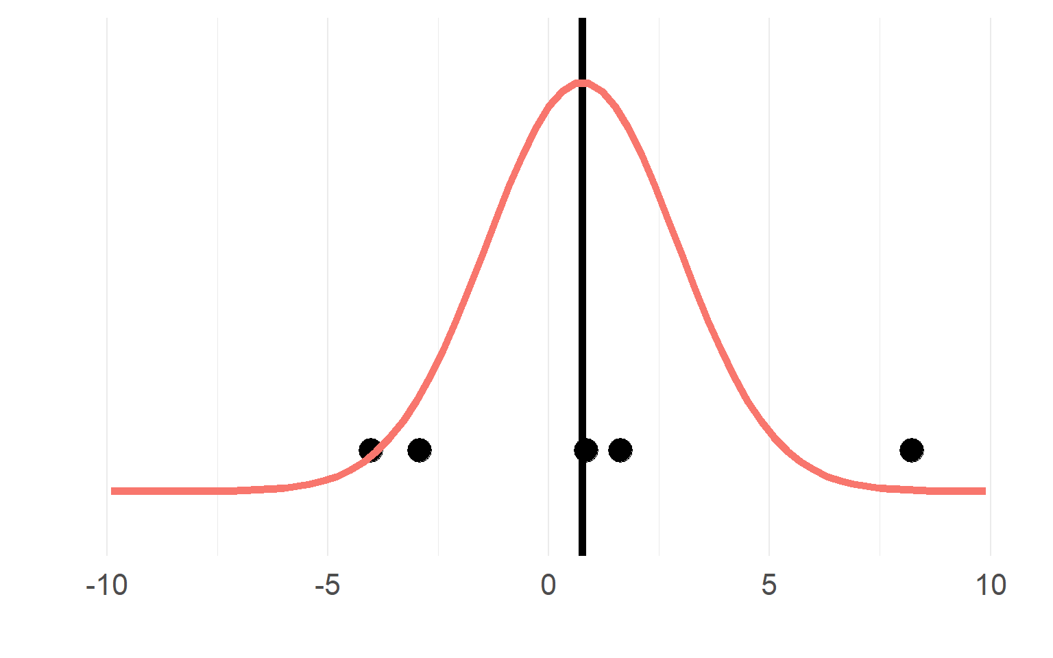
 with \(n_T =15\) trials
 This sampling distribution reflects these exact 5 subjects. But does not generalize!
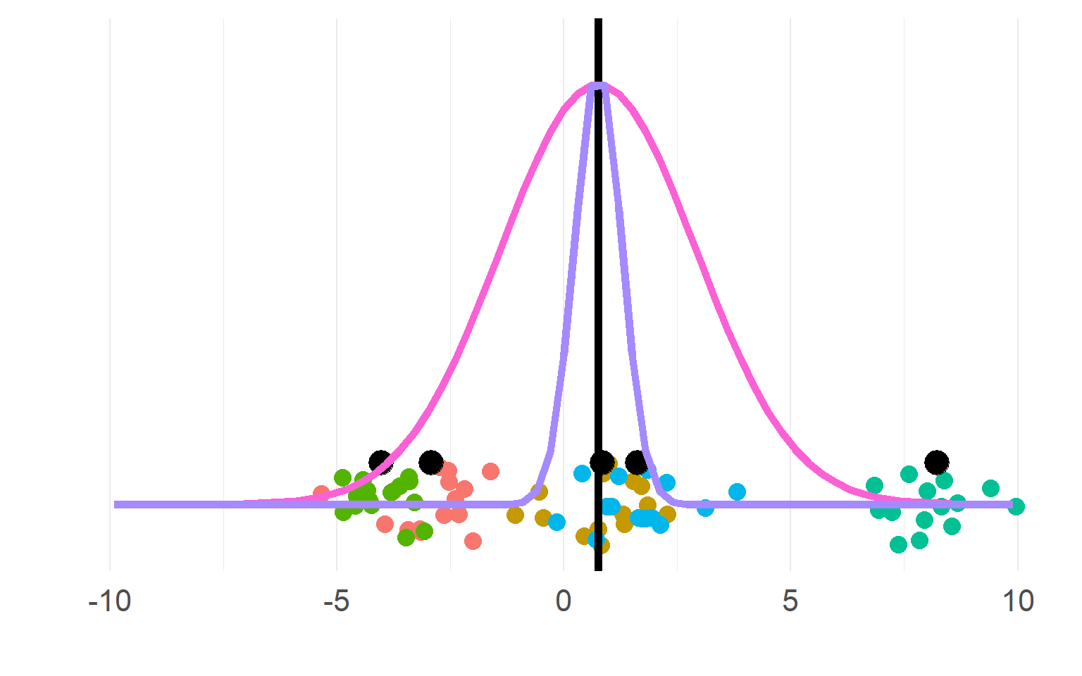 (pink for aggregate, purple for disaggregate). There is a strong allure to choose the purple one, easier to get significant results!
  \[\sigma_{within} >> \sigma_{between}\]
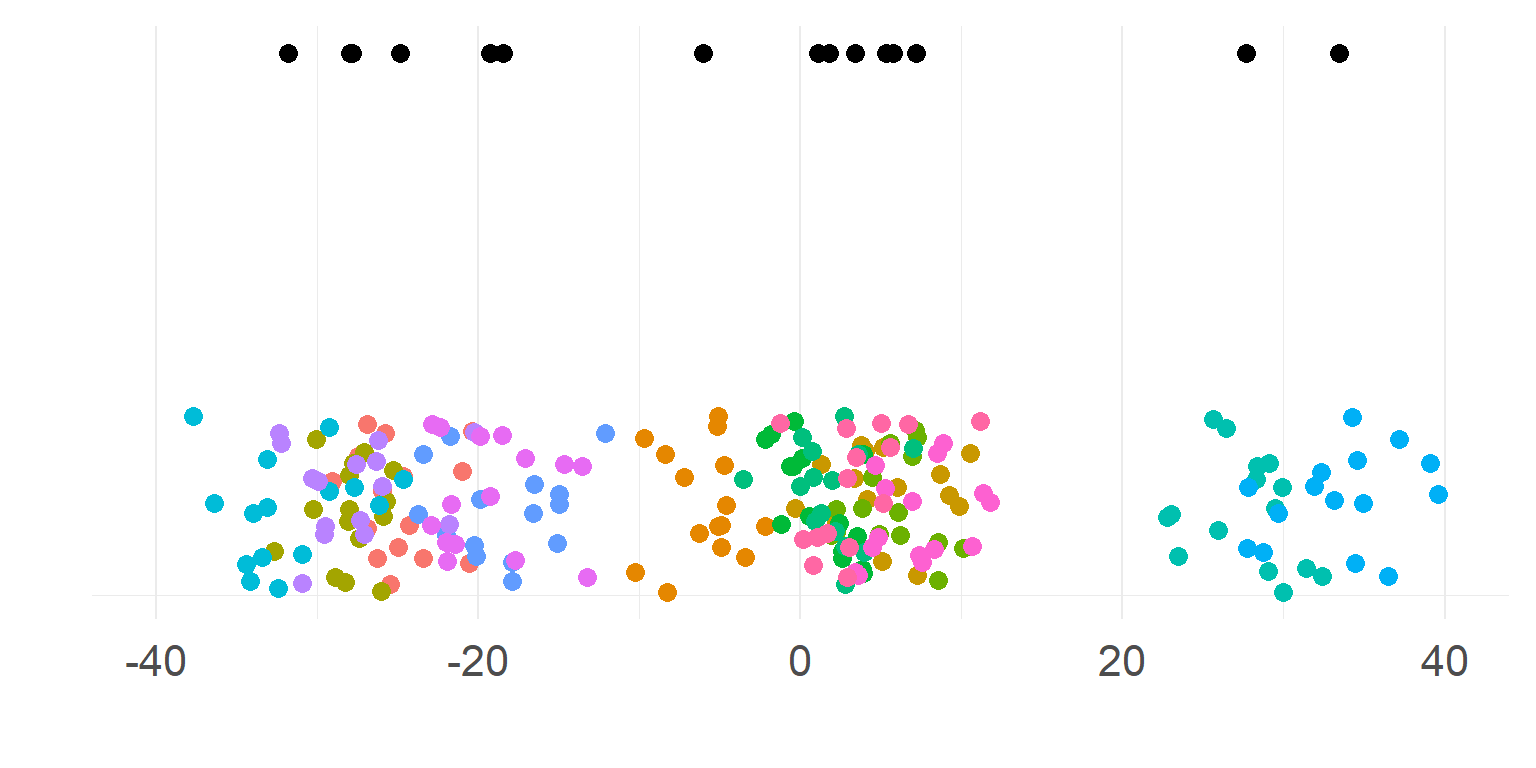 \[\sigma_{within} << \sigma_{between}\]
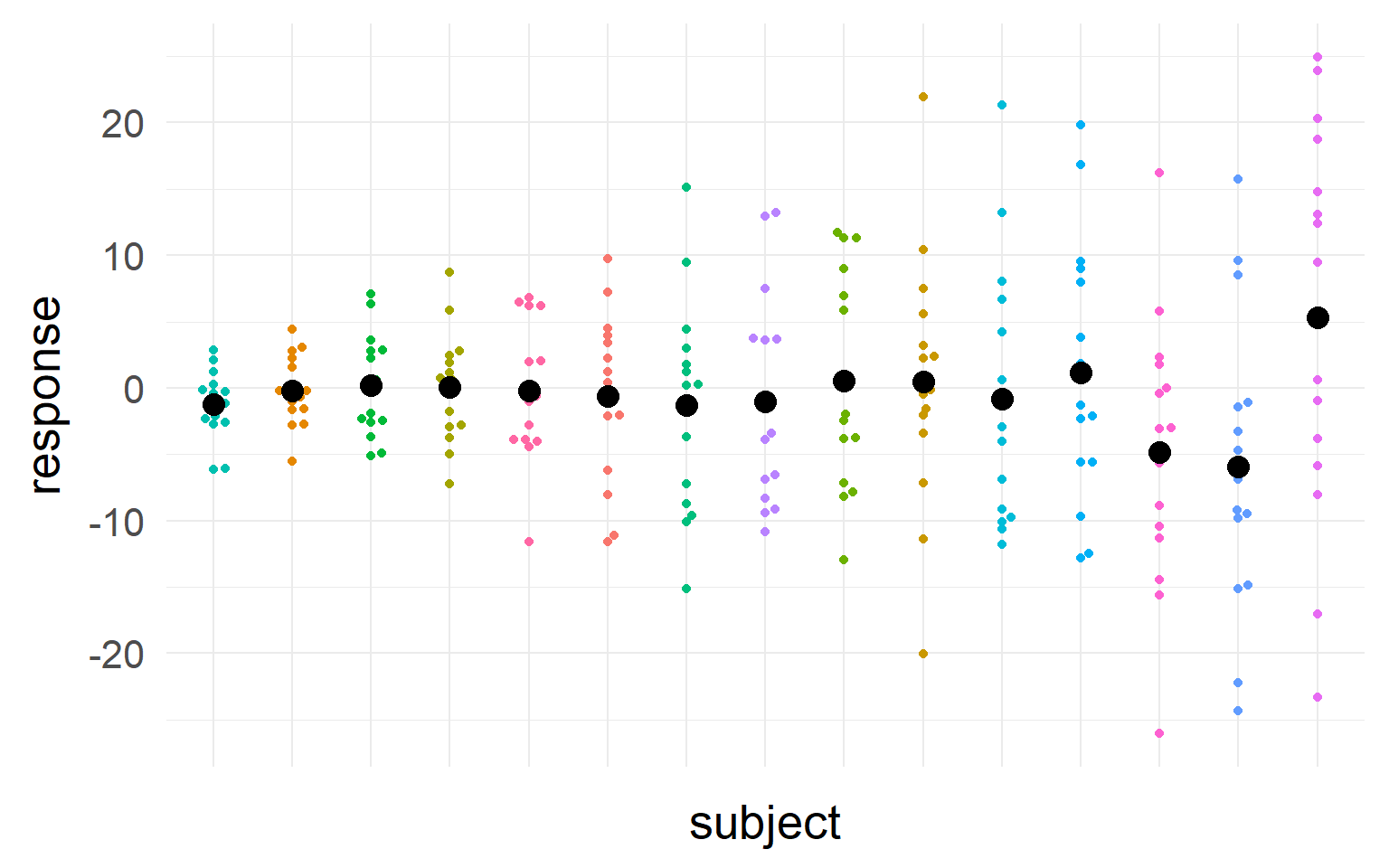


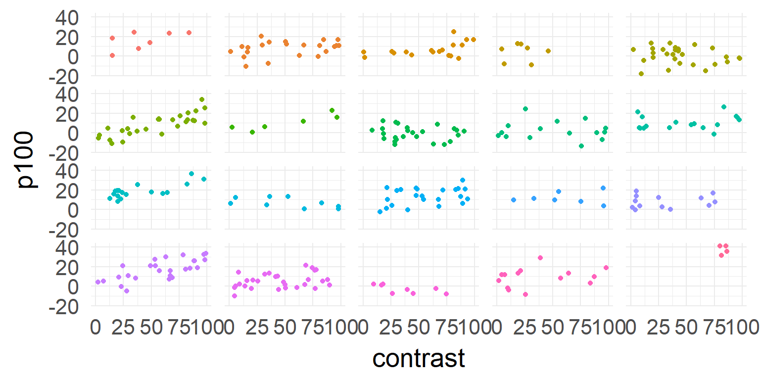
 \[\hat{y} = \beta_0 + \beta_1 * contrast \]
 \[\hat{y_j} = \beta_{0,j} + \beta_{1,j} * contrast \]
 Linear Mixed Model aka Hierarchical Model aka Multilevel Model
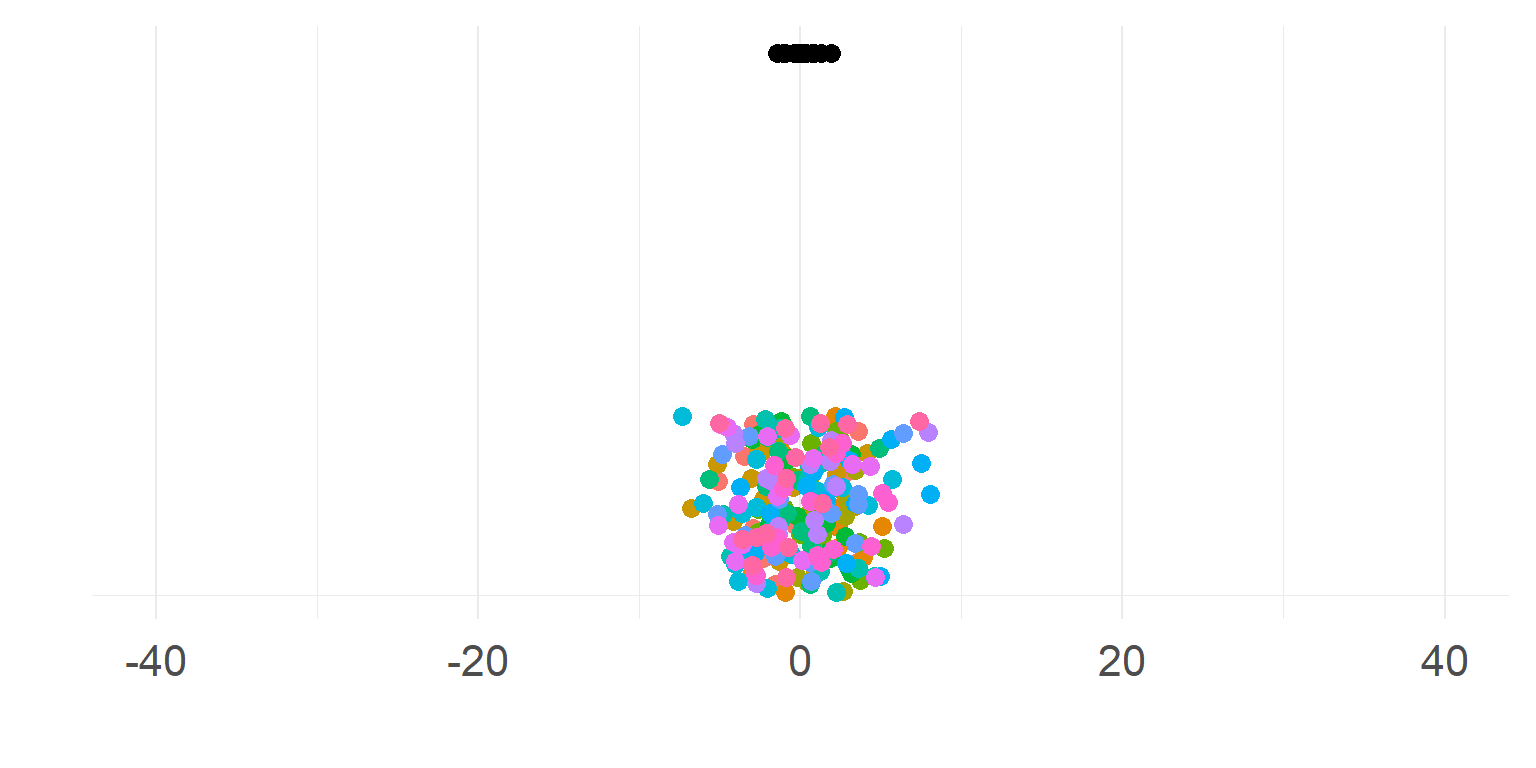


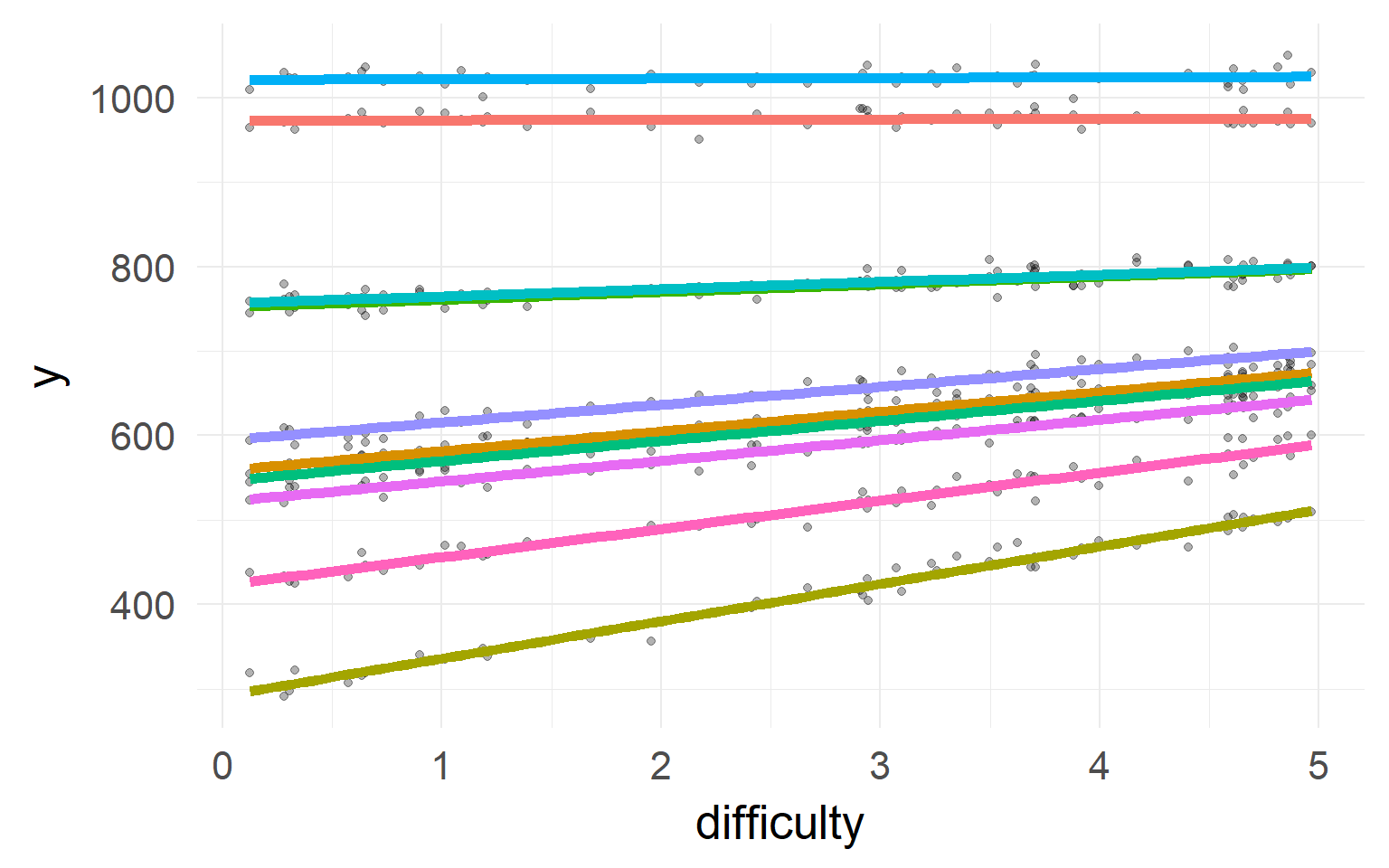 Simulated data: Subjects with faster reaction time (intercept) show larger effects for difficulty (slope)
 \(\rho = 0\), knowing one dimension does not tell you about the other
 \(\rho = 0.6\), knowing one dimension tells you something about the other