Logistic Regression: Will it rain in Osnabrück tomorrow?
TLDR;
52% of days it rained (Precipitation>0)
Is it sunny? 2x as likely that it is sunny tomorrow as well.
Is it rainy? 2.3x as likely that it is rainy tomorrow as well
Predicting rainfall using logistic regression
I’m playing around with some analyses for an upcoming course. This follows loosely the example of “Advanced Data Analysis from an Elemental Point of View” Chapter 12.7
It is a somewhat naive analysis. Further improvements are discussed at the end.
library(ggplot2)
library(plyr)
We load the data and change some of the German variables
# I downloaded the data from here:
# http://www.dwd.de/DE/leistungen/klimadatendeutschland/klimadatendeutschland.html
weather = data.frame(read.csv(file='produkt_klima_Tageswerte_19891001_20151231_01766.txt',sep=';'))
weather$date = as.Date.character(x=weather$MESS_DATUM,format="%Y%m%d")
weather = rename(weather,replace = c("NIEDERSCHLAGSHOEHE"="rain"))
weather$rain_tomorrow = c(tail(weather$rain,-1),NA)

weather <- weather[-nrow(weather),] # remove NA row
summary(weather[,c("date","rain","rain_tomorrow")])
##       date                 rain         rain_tomorrow
##  Min.   :1989-10-01   Min.   :  0.000   Min.   :  0.000
##  1st Qu.:1996-04-23   1st Qu.:  0.000   1st Qu.:  0.000
##  Median :2002-11-15   Median :  0.100   Median :  0.100
##  Mean   :2002-11-15   Mean   :  2.055   Mean   :  2.055
##  3rd Qu.:2009-06-07   3rd Qu.:  2.200   3rd Qu.:  2.200
##  Max.   :2015-12-30   Max.   :140.100   Max.   :140.100
The data range from 1989 up until the end of 2015.
p1= ggplot(weather,aes(x=rain))+geom_density()
cowplot::plot_grid(p1,p1+scale_x_log10())
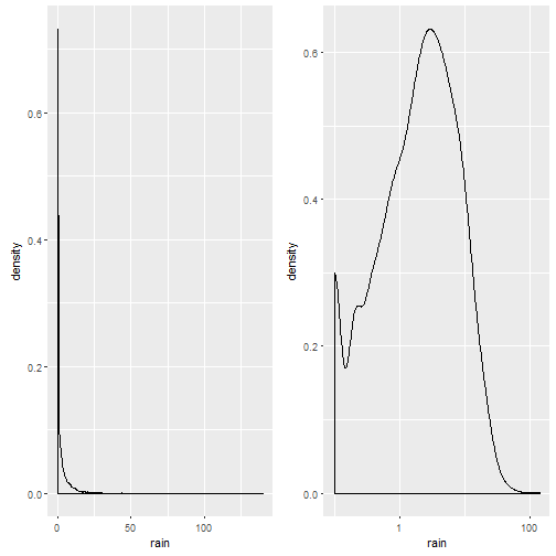
Notice that the plot on the left is in native scale, the one on the right in x-axis-log-scale.
We take the mean of rainy days (ml/day > 0): There is a 52% probability it will rain on a given day (what everyone living in Osnabrück already knew, it rains more often than not).
Predicting rain from the day before
For exercise reasons I made several logistic regressions. I try to predict whether there will be rain on the day afterwards, based on the amount of rain on the current day.
m.weather.1 = glm(formula = rain_tomorrow>0 ~ rain>0,data=weather,family = "binomial")
summary(m.weather.1)
##
## Call:
## glm(formula = rain_tomorrow > 0 ~ rain > 0, family = "binomial",
##     data = weather)
##
## Deviance Residuals:
##     Min       1Q   Median       3Q      Max
## -1.5431  -0.8889   0.8514   0.8514   1.4965
##
## Coefficients:
##              Estimate Std. Error z value Pr(>|z|)
## (Intercept)  -0.72478    0.03136  -23.11   <2e-16 ***
## rain > 0TRUE  1.55287    0.04400   35.29   <2e-16 ***
## ---
## Signif. codes:  0 '***' 0.001 '**' 0.01 '*' 0.05 '.' 0.1 ' ' 1
##
## (Dispersion parameter for binomial family taken to be 1)
##
##     Null deviance: 13278  on 9586  degrees of freedom
## Residual deviance: 11938  on 9585  degrees of freedom
## AIC: 11942
##
## Number of Fisher Scoring iterations: 4
Whoop Whoop, Wald’s t-value of ~35! Keep in mind that the predictor values are in logit-space. That means, a predictor value of -0.72 is a log-odd value. In order to calculate this back to an easier interpreted format, we can simply take the exponential and receive the odds-ratio.
Do the calculations:
exp(coef(m.weather.1)[1])
## (Intercept)
##   0.4844302
exp(sum(coef(m.weather.1))) # the odds for rain tomorrow if it is rainy (2 : 1)
## [1] 2.288933
Now we can interprete the odds:
The odds of rain tomorrow if there was a sunny day are 0.5:1, i.e. it is double as likely that the next day is sunny, if it was sunny today
The odds of rain tomorrow if it was a rainy day are 2.3:1, i.e. it is more than double as likely that the next day is rainy, if it was rainy today.
Can we get better?
We could try to predict rain based on the daily continuous precipitation (in ml).
We will compare this with the previous model using BIC (smaller number => better model).
m.weather.2 = glm(formula = rain_tomorrow>0 ~ rain,data=weather,family="binomial")
BIC(m.weather.1,m.weather.2)
##             df      BIC
## m.weather.1  2 11956.09
## m.weather.2  2 12505.85
Turns out: No, a categorical model (is there rain today, or not?) beats the continuous one. But why?
d.predNew = data.frame(rain=seq(0,50));
d.pred=             cbind(d.predNew,pred=arm::invlogit(predict(m.weather.2,newdata = d.predNew)),model='2')
d.pred=rbind(d.pred,cbind(d.predNew,pred=arm::invlogit(predict(m.weather.1,newdata = d.predNew)),model='1'))

p1 = ggplot()+geom_point(data=d.pred,aes(x=rain,y=pred,color=model) )+
    geom_smooth(data=weather,aes(x=rain,y=(rain_tomorrow>0)*1))
cowplot::plot_grid(p1,p1+scale_x_log10())
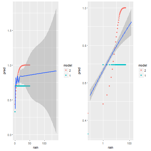
We plot the predictions model 1 does in green, model 2 in red and the smoothed data in blue. On the left we have the x-axis in native units [ml?] on the right on log-scale. It is very clear, that the red dots do not match the empirical data (blue) at all. The green dots (model 1) are better. My guess is, this is due to some outlier influencing the slope, but also due to the non-homogenious distribution of rain-values as seen i the first figure
We will try two transformations off X (a log effect seems possible?)
- sqrt(rain)
- log(rain+0.001)
m.weather.3 = glm(formula = rain_tomorrow>0 ~ sqrt(rain),data=weather,family="binomial")
# Box-Cox transform with lambda2 = 0.001 http://robjhyndman.com/hyndsight/transformations/
m.weather.4 = glm(formula = rain_tomorrow>0 ~ log(rain+0.001),data=weather,family="binomial")


BIC(m.weather.1,m.weather.2,m.weather.3,m.weather.4)
##             df      BIC
## m.weather.1  2 11956.09
## m.weather.2  2 12505.85
## m.weather.3  2 12020.09
## m.weather.4  2 11795.15
It is surprisingly hard to beat the simple first model, but in the end – we did it! The log(rain) model seems to capture the data best.
d.predNew = data.frame(rain=seq(0,50));
d.pred=             cbind(d.predNew,pred=arm::invlogit(predict(m.weather.4,newdata = d.predNew)),model='2')
d.pred=rbind(d.pred,cbind(d.predNew,pred=arm::invlogit(predict(m.weather.1,newdata = d.predNew)),model='1'))
d.pred=rbind(d.pred,cbind(d.predNew,pred=arm::invlogit(predict(m.weather.3,newdata = d.predNew)),model='3'))
d.pred=rbind(d.pred,cbind(d.predNew,pred=arm::invlogit(predict(m.weather.4,newdata = d.predNew)),model='4'))

p1 = ggplot()+geom_point(data=d.pred,aes(x=rain,y=pred,color=model) )+
    geom_smooth(data=weather,aes(x=rain,y=(rain_tomorrow>0)*1))
cowplot::plot_grid(p1,p1+scale_x_log10())
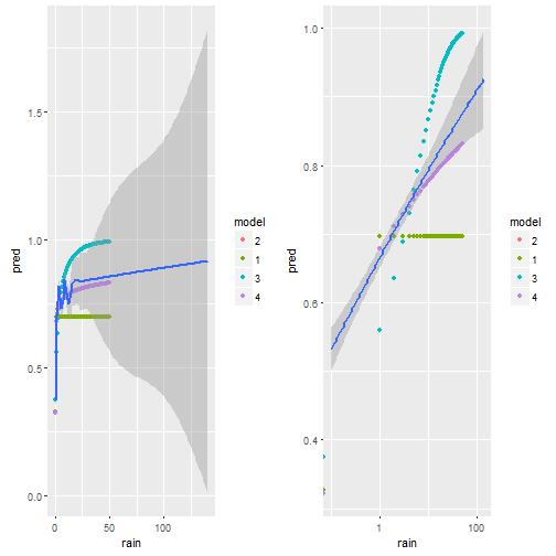
Visually we can see that model 4 comes the non-linear smoother the closest.
Improvements
- use nonlinear effects (GAM) as done in the book
- multivariate (make use of the plentitude of other information as well)
- use the months as a cyclical predictor, i.e. seasonal trends will be clearly present in the data
Misc
This post was directly exported using knit2wp and R-Markdown. It works kind of okay, but clearly the figures are not wide enough, even though I specify the correct width in the markdown. I might upload them later manually.